Analysis of variance

[1] These include hypothesis testing, the partitioning of sums of squares, experimental techniques and the additive model.

[8] Ronald Fisher introduced the term variance and proposed its formal analysis in a 1918 article on theoretical population genetics, The Correlation Between Relatives on the Supposition of Mendelian Inheritance.

[11] Analysis of variance became widely known after being included in Fisher's 1925 book Statistical Methods for Research Workers.

Teaching experiments could be performed by a college or university department to find a good introductory textbook, with each text considered a treatment.

The random-effects model would determine whether important differences exist among a list of randomly selected texts.

[14] The analysis of variance has been studied from several approaches, the most common of which uses a linear model that relates the response to the treatments and blocks.

The objective random-assignment is used to test the significance of the null hypothesis, following the ideas of C. S. Peirce and Ronald Fisher.

This design-based analysis was discussed and developed by Francis J. Anscombe at Rothamsted Experimental Station and by Oscar Kempthorne at Iowa State University.

The use of unit treatment additivity and randomization is similar to the design-based inference that is standard in finite-population survey sampling.

However, when applied to data from non-randomized experiments or observational studies, model-based analysis lacks the warrant of randomization.

[29] For observational data, the derivation of confidence intervals must use subjective models, as emphasized by Ronald Fisher and his followers.

In practice, "statistical models" and observational data are useful for suggesting hypotheses that should be treated very cautiously by the public.

[30] The normal-model based ANOVA analysis assumes the independence, normality, and homogeneity of variances of the residuals.

The randomization-based analysis assumes only the homogeneity of the variances of the residuals (as a consequence of unit-treatment additivity) and uses the randomization procedure of the experiment.

However, studies of processes that change variances rather than means (called dispersion effects) have been successfully conducted using ANOVA.

[32] Also, a statistician may specify that logarithmic transforms be applied to the responses which are believed to follow a multiplicative model.

So ANOVA statistical significance result is independent of constant bias and scaling errors as well as the units used in expressing observations.

In the era of mechanical calculation it was common to subtract a constant from all observations (when equivalent to dropping leading digits) to simplify data entry.

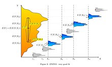
The fundamental technique is a partitioning of the total sum of squares SS into components related to the effects used in the model.

There are two methods of concluding the ANOVA hypothesis test, both of which produce the same result: The ANOVA F-test is known to be nearly optimal in the sense of minimizing false negative errors for a fixed rate of false positive errors (i.e. maximizing power for a fixed significance level).

[nb 2] The ANOVA F-test (of the null-hypothesis that all treatments have exactly the same effect) is recommended as a practical test, because of its robustness against many alternative distributions.

[38][nb 3] ANOVA consists of separable parts; partitioning sources of variance and hypothesis testing can be used individually.

where That is, we envision an additive model that says every data point can be represented by summing three quantities: the true mean, averaged over all factor levels being investigated, plus an incremental component associated with the particular column (factor level), plus a final component associated with everything else affecting that specific data value.

The proliferation of interaction terms increases the risk that some hypothesis test will produce a false positive by chance.

[41] [verification needed] The ability to detect interactions is a major advantage of multiple factor ANOVA.

Testing one factor at a time hides interactions, but produces apparently inconsistent experimental results.

"[45] The analysis, which is written in the experimental protocol before the experiment is conducted, is examined in grant applications and administrative review boards.

[52] Residuals should have the appearance of (zero mean normal distribution) noise when plotted as a function of anything including time and modeled data values.

Comparisons can also look at tests of trend, such as linear and quadratic relationships, when the independent variable involves ordered levels.

"The orthogonality property of main effects and interactions present in balanced data does not carry over to the unbalanced case.