Analytical mechanics
Analytical mechanics takes advantage of a system's constraints to solve problems.
The constraints limit the degrees of freedom the system can have, and can be used to reduce the number of coordinates needed to solve for the motion.
The kinetic and potential energies of the system are expressed using these generalized coordinates or momenta, and the equations of motion can be readily set up, thus analytical mechanics allows numerous mechanical problems to be solved with greater efficiency than fully vectorial methods.
Both formulations are equivalent by a Legendre transformation on the generalized coordinates, velocities and momenta; therefore, both contain the same information for describing the dynamics of a system.
All equations of motion for particles and fields, in any formalism, can be derived from the widely applicable result called the principle of least action.
Analytical mechanics is used widely, from fundamental physics to applied mathematics, particularly chaos theory.
The methods of analytical mechanics apply to discrete particles, each with a finite number of degrees of freedom.
Starting from a physical system—such as a mechanism or a star system—a mathematical model is developed in the form of a differential equation.
Newton's vectorial approach to mechanics describes motion with the help of vector quantities such as force, velocity, acceleration.
Using a Newtonian approach is possible, under proper precautions, namely isolating each single particle from the others, and determining all the forces acting on it.
Newton thought that his third law "action equals reaction" would take care of all complications.
[clarification needed] In more complicated systems, the vectorial approach cannot give an adequate description.
However, the analytical treatment does not require the knowledge of these forces and takes these kinematic conditions for granted.
[citation needed] Still, deriving the equations of motion of a complicated mechanical system requires a unifying basis from which they follow.
A problem is regarded as solved when the particles coordinates at time t are expressed as simple functions of t and of parameters defining the initial positions and velocities.
It concentrates on systems to which Lagrangian or Hamiltonian equations of motion are applicable and that include a very wide range of problems indeed.
[3] Development of analytical mechanics has two objectives: (i) increase the range of solvable problems by developing standard techniques with a wide range of applicability, and (ii) understand the mathematical structure of mechanics.
There is one generalized coordinate qi for each degree of freedom (for convenience labelled by an index i = 1, 2...N), i.e. each way the system can change its configuration; as curvilinear lengths or angles of rotation.
[5] The introduction of generalized coordinates and the fundamental Lagrangian function: where T is the total kinetic energy and V is the total potential energy of the entire system, then either following the calculus of variations or using the above formula – lead to the Euler–Lagrange equations; which are a set of N second-order ordinary differential equations, one for each qi(t).
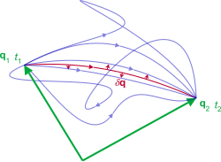
This formulation identifies the actual path followed by the motion as a selection of the path over which the time integral of kinetic energy is least, assuming the total energy to be fixed, and imposing no conditions on the time of transit.
The Lagrangian formulation uses the configuration space of the system, the set of all possible generalized coordinates: where
The particular solution to the Euler–Lagrange equations is called a (configuration) path or trajectory, i.e. one particular q(t) subject to the required initial conditions.
Another result from the Legendre transformation relates the time derivatives of the Lagrangian and Hamiltonian: which is often considered one of Hamilton's equations of motion additionally to the others.
A particular solution to Hamilton's equations is called a phase path, a particular curve (q(t),p(t)) subject to the required initial conditions.
If A(q, p, t) and B(q, p, t) are two scalar valued dynamical variables, the Poisson bracket is defined by the generalized coordinates and momenta: Calculating the total derivative of one of these, say A, and substituting Hamilton's equations into the result leads to the time evolution of A: This equation in A is closely related to the equation of motion in the Heisenberg picture of quantum mechanics, in which classical dynamical variables become quantum operators (indicated by hats (^)), and the Poisson bracket is replaced by the commutator of operators via Dirac's canonical quantization: Following are overlapping properties between the Lagrangian and Hamiltonian functions.
This approach can be extended to fields rather than a system of particles (see below), and underlies the path integral formulation of quantum mechanics,[11][12] and is used for calculating geodesic motion in general relativity.
) plus an arbitrary constant C: the generalized momenta become: and P is constant, then the Hamiltonian-Jacobi equation (HJE) can be derived from the type-2 canonical transformation: where H is the Hamiltonian as before: Another related function is Hamilton's characteristic function used to solve the HJE by additive separation of variables for a time-independent Hamiltonian H. The study of the solutions of the Hamilton–Jacobi equations leads naturally to the study of symplectic manifolds and symplectic topology.
Set up in this way, although the Routhian has the form of the Hamiltonian, it can be thought of a Lagrangian with N − s degrees of freedom.
Each transformation can be described by an operator (i.e. function acting on the position r or momentum p variables to change them).
[11] where R(n̂, θ) is the rotation matrix about an axis defined by the unit vector n̂ and angle θ. Noether's theorem states that a continuous symmetry transformation of the action corresponds to a conservation law, i.e. the action (and hence the Lagrangian) does not change under a transformation parameterized by a parameter s: