Atmospheric dispersion modeling
It is performed with computer programs that include algorithms to solve the mathematical equations that govern the pollutant dispersion.
The dispersion models are used to estimate the downwind ambient concentration of air pollutants or toxins emitted from sources such as industrial plants, vehicular traffic or accidental chemical releases.
For pollutants that have a very high spatio-temporal variability (i.e. have very steep distance to source decay such as black carbon) and for epidemiological studies statistical land-use regression models are also used.
Dispersion models are important to governmental agencies tasked with protecting and managing the ambient air quality.
The models also serve to assist in the design of effective control strategies to reduce emissions of harmful air pollutants.
During the late 1960s, the Air Pollution Control Office of the U.S. EPA initiated research projects that would lead to the development of models for the use by urban and transportation planners.
[1] A major and significant application of a roadway dispersion model that resulted from such research was applied to the Spadina Expressway of Canada in 1971.
The results of dispersion modeling, using worst case accidental release source terms and meteorological conditions, can provide an estimate of location impacted areas, ambient concentrations, and be used to determine protective actions appropriate in the event a release occurs.
Appropriate protective actions may include evacuation or shelter in place for persons in the downwind direction.
At industrial facilities, this type of consequence assessment or emergency planning is required under the U.S. Clean Air Act (CAA) codified in Part 68 of Title 40 of the Code of Federal Regulations.
The dispersion models vary depending on the mathematics used to develop the model, but all require the input of data that may include: Many of the modern, advanced dispersion modeling programs include a pre-processor module for the input of meteorological and other data, and many also include a post-processor module for graphing the output data and/or plotting the area impacted by the air pollutants on maps.
We call the region of the PBL below its capping inversion the convective planetary boundary layer; it is typically 1.5 to 2 km (0.93 to 1.24 mi) in height.
In tropical and mid-latitudes during daytime, the free convective layer can comprise the entire troposphere, which is up to 10 to 18 km (6.2 to 11.2 mi) in the Intertropical Convergence Zone.
The PBL is important with respect to the transport and dispersion of airborne pollutants because the turbulent dynamics of wind are strongest at Earth's surface.
Almost all of the airborne pollutants emitted into the ambient atmosphere are transported and dispersed within the mixing layer.
The technical literature on air pollution dispersion is quite extensive and dates back to the 1930s and earlier.
One of the early air pollutant plume dispersion equations was derived by Bosanquet and Pearson.
[2] Their equation did not assume Gaussian distribution nor did it include the effect of ground reflection of the pollutant plume.
Under the stimulus provided by the advent of stringent environmental control regulations, there was an immense growth in the use of air pollutant plume dispersion calculations between the late 1960s and today.
[8] The six stability classes are referred to: A-extremely unstable B-moderately unstable C-slightly unstable D-neutral E-slightly stable F-moderately stable The resulting calculations for air pollutant concentrations are often expressed as an air pollutant concentration contour map in order to show the spatial variation in contaminant levels over a wide area under study.
In this way the contour lines can overlay sensitive receptor locations and reveal the spatial relationship of air pollutants to areas of interest.
Whereas older models rely on stability classes (see air pollution dispersion terminology) for the determination of
, more recent models increasingly rely on the Monin-Obukhov similarity theory to derive these parameters.
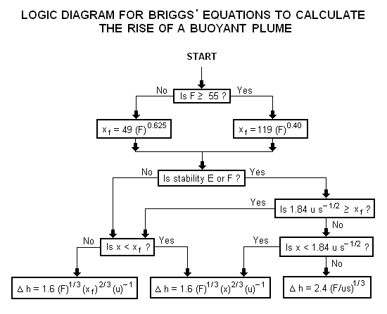
To determine ΔH, many if not most of the air dispersion models developed between the late 1960s and the early 2000s used what are known as the Briggs equations.
[9] In 1968, at a symposium sponsored by CONCAWE (a Dutch organization), he compared many of the plume rise models then available in the literature.
[10] In that same year, Briggs also wrote the section of the publication edited by Slade[11] dealing with the comparative analyses of plume rise models.
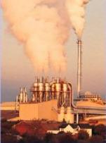
In general, Briggs's equations for bent-over, hot buoyant plumes are based on observations and data involving plumes from typical combustion sources such as the flue gas stacks from steam-generating boilers burning fossil fuels in large power plants.