Curvilinear coordinates

Curvilinear coordinates are often used to define the location or distribution of physical quantities which may be, for example, scalars, vectors, or tensors.

Mathematical expressions involving these quantities in vector calculus and tensor analysis (such as the gradient, divergence, curl, and Laplacian) can be transformed from one coordinate system to another, according to transformation rules for scalars, vectors, and tensors.

A point P in 3-D space (or its position vector r) can be defined using Cartesian coordinates (x, y, z) [equivalently written (x1, x2, x3)], by

Basis vectors that are the same at all points are global bases, and can be associated only with linear or affine coordinate systems.

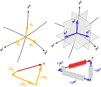
In the case that they are orthogonal at all points where the derivatives are well-defined, we define the Lamé coefficients (after Gabriel Lamé) by and the curvilinear orthonormal basis vectors by These basis vectors may well depend upon the position of P; it is therefore necessary that they are not assumed to be constant over a region.

at P, and so are local to P.) In general, curvilinear coordinates allow the natural basis vectors hi not all mutually perpendicular to each other, and not required to be of unit length: they can be of arbitrary magnitude and direction.

The six independent scalar products gij=hi.hj of the natural basis vectors generalize the three scale factors defined above for orthogonal coordinates.

Spatial gradients, distances, time derivatives and scale factors are interrelated within a coordinate system by two groups of basis vectors: Note that, because of Einstein's summation convention, the position of the indices of the vectors is the opposite of that of the coordinates.

The covariant and contravariant basis vectors types have identical direction for orthogonal curvilinear coordinate systems, but as usual have inverted units with respect to each other.

By the chain rule, dq1 can be expressed as: If the displacement dr is such that dq2 = dq3 = 0, i.e. the position vector r moves by an infinitesimal amount along the coordinate axis q2=const and q3=const, then: Dividing by dq1, and taking the limit dq1 → 0: or equivalently: Now if the displacement dr is such that dq1=dq3=0, i.e. the position vector r moves by an infinitesimal amount along the coordinate axis q1=const and q3=const, then: Dividing by dq2, and taking the limit dq2 → 0: or equivalently: And so forth for the other dot products.

It can be seen from triangle PAB that where |e1|, |b1| are the magnitudes of the two basis vectors, i.e., the scalar intercepts PB and PA. PA is also the projection of b1 on the x axis.

However, this method for basis vector transformations using directional cosines is inapplicable to curvilinear coordinates for the following reasons: The angles that the q1 line and that axis form with the x axis become closer in value the closer one moves towards point P and become exactly equal at P. Let point E be located very close to P, so close that the distance PE is infinitesimally small.

Then Thus, the directional cosines can be substituted in transformations with the more exact ratios between infinitesimally small coordinate intercepts.

In three dimensions, the expanded forms of these matrices are In the inverse transformation (second equation system), the unknowns are the curvilinear basis vectors.

Each vector has exactly one component in each dimension (or "axis") and they are mutually orthogonal (perpendicular) and normalized (has unit magnitude).

With this simple definition of a curvilinear coordinate system, all the results that follow below are simply applications of standard theorems in differential topology.

The transformation functions are such that there's a one-to-one relationship between points in the "old" and "new" coordinates, that is, those functions are bijections, and fulfil the following requirements within their domains: Elementary vector and tensor algebra in curvilinear coordinates is used in some of the older scientific literature in mechanics and physics and can be indispensable to understanding work from the early and mid-1900s, for example the text by Green and Zerna.

The notation and contents are primarily from Ogden,[6] Naghdi,[7] Simmonds,[2] Green and Zerna,[5] Basar and Weichert,[8] and Ciarlet.

The components of the second-order tensor are related by At each point, one can construct a small line element dx, so the square of the length of the line element is the scalar product dx • dx and is called the metric of the space, given by: The following portion of the above equation is a symmetric tensor called the fundamental (or metric) tensor of the Euclidean space in curvilinear coordinates.

In curvilinear coordinates, the equivalent expression is Adjustments need to be made in the calculation of line, surface and volume integrals.

Simmonds,[2] in his book on tensor analysis, quotes Albert Einstein saying[10] The magic of this theory will hardly fail to impose itself on anybody who has truly understood it; it represents a genuine triumph of the method of absolute differential calculus, founded by Gauss, Riemann, Ricci, and Levi-Civita.

Vector and tensor calculus in general curvilinear coordinates is used in tensor analysis on four-dimensional curvilinear manifolds in general relativity,[11] in the mechanics of curved shells,[9] in examining the invariance properties of Maxwell's equations which has been of interest in metamaterials[12][13] and in many other fields.

The notation and contents are primarily from Ogden,[14] Simmonds,[2] Green and Zerna,[5] Basar and Weichert,[8] and Ciarlet.

In determinant form: The expressions for the gradient, divergence, and Laplacian can be directly extended to n-dimensions, however the curl is only defined in 3D.

By definition, if a particle with no forces acting on it has its position expressed in an inertial coordinate system, (x1, x2, x3, t), then there it will have no acceleration (d2xj/dt2 = 0).

Strictly speaking, these terms represent components of the absolute acceleration (in classical mechanics), but we may also choose to continue to regard d2xj/dt2 as the acceleration (as if the coordinates were inertial) and treat the extra terms as if they were forces, in which case they are called fictitious forces.

[18][19][20]) For a simple example, consider a particle of mass m moving in a circle of radius r with angular speed w relative to a system of polar coordinates rotating with angular speed W. The radial equation of motion is mr” = Fr + mr(w + W)2.

Thus the centrifugal force is mr times the square of the absolute rotational speed A = w + W of the particle.

The reason for this equality of results is that in both cases the basis vectors at the particle's location are changing in time in exactly the same way.

When describing general motion, the actual forces acting on a particle are often referred to the instantaneous osculating circle tangent to the path of motion, and this circle in the general case is not centered at a fixed location, and so the decomposition into centrifugal and Coriolis components is constantly changing.