Data parallelism

It can be applied on regular data structures like arrays and matrices by working on each element in parallel.

A data parallel job on an array of n elements can be divided equally among all the processors.

Locality of data depends on the memory accesses performed by the program as well as the size of the cache.

Exploitation of the concept of data parallelism started in 1960s with the development of the Solomon machine.

[1] The Solomon machine, also called a vector processor, was developed to expedite the performance of mathematical operations by working on a large data array (operating on multiple data in consecutive time steps).

We can exploit data parallelism in the preceding code to execute it faster as the arithmetic is loop independent.

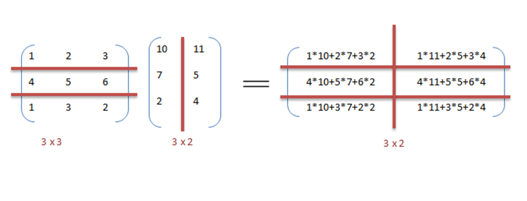
It can be observed from the example that a lot of processors will be required as the matrix sizes keep on increasing.

Keeping the execution time low is the priority but as the matrix size increases, we are faced with other constraints like complexity of such a system and its associated costs.

Therefore, constraining the number of processors in the system, we can still apply the same principle and divide the data into bigger chunks to calculate the product of two matrices.

The program expressed in pseudocode below—which applies some arbitrary operation, foo, on every element in the array d—illustrates data parallelism:[nb 1] In an SPMD system executed on 2 processor system, both CPUs will execute the code.

Mixed parallelism requires sophisticated scheduling algorithms and software support.

It is particularly used in the following applications: A variety of data parallel programming environments are available today, most widely used of which are: Data parallelism finds its applications in a variety of fields ranging from physics, chemistry, biology, material sciences to signal processing.