Discrete cosine transform

The DCT, first proposed by Nasir Ahmed in 1972, is a widely used transformation technique in signal processing and data compression.

The DCT was first conceived by Nasir Ahmed, T. Natarajan and K. R. Rao while working at Kansas State University.

[9][1] Ahmed developed a practical DCT algorithm with his PhD students T. Raj Natarajan, Wills Dietrich, and Jeremy Fries, and his friend Dr. K. R. Rao at the University of Texas at Arlington in 1973.

[10] In 1977, Wen-Hsiung Chen published a paper with C. Harrison Smith and Stanley C. Fralick presenting a fast DCT algorithm.

[13] In 1975, John A. Roese and Guner S. Robinson adapted the DCT for inter-frame motion-compensated video coding.

They experimented with the DCT and the fast Fourier transform (FFT), developing inter-frame hybrid coders for both, and found that the DCT is the most efficient due to its reduced complexity, capable of compressing image data down to 0.25-bit per pixel for a videotelephone scene with image quality comparable to an intra-frame coder requiring 2-bit per pixel.

[17] This led to Chen developing a practical video compression algorithm, called motion-compensated DCT or adaptive scene coding, in 1981.

[18][19] A DCT variant, the modified discrete cosine transform (MDCT), was developed by John P. Princen, A.W.

[26] Nasir Ahmed also developed a lossless DCT algorithm with Giridhar Mandyam and Neeraj Magotra at the University of New Mexico in 1995.

[7][35] The DCT, and in particular the DCT-II, is often used in signal and image processing, especially for lossy compression, because it has a strong energy compaction property.

For strongly correlated Markov processes, the DCT can approach the compaction efficiency of the Karhunen-Loève transform (which is optimal in the decorrelation sense).

[89] Due to enhancement in the hardware, software and introduction of several fast algorithms, the necessity of using MD DCTs is rapidly increasing.

DCT-IV has gained popularity for its applications in fast implementation of real-valued polyphase filtering banks,[90] lapped orthogonal transform[91][92] and cosine-modulated wavelet bases.

[93] DCT plays an important role in digital signal processing specifically data compression.

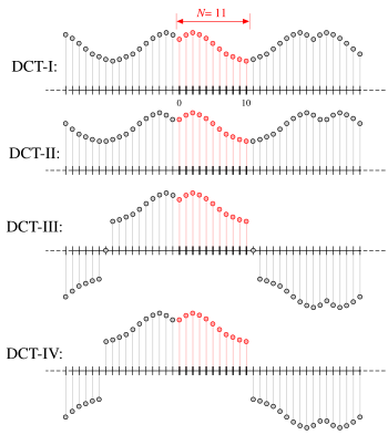
[97][98] Like any Fourier-related transform, DCTs express a function or a signal in terms of a sum of sinusoids with different frequencies and amplitudes.

However, because DCTs operate on finite, discrete sequences, two issues arise that do not apply for the continuous cosine transform.

These different boundary conditions strongly affect the applications of the transform and lead to uniquely useful properties for the various DCT types.

This makes the DCT-II matrix orthogonal, but breaks the direct correspondence with a real-even DFT of half-shifted input.

This makes the DCT-III matrix orthogonal, but breaks the direct correspondence with a real-even DFT of half-shifted output.

The four additional types of discrete cosine transform[104] correspond essentially to real-even DFTs of logically odd order, which have factors of

Multidimensional variants of the various DCT types follow straightforwardly from the one-dimensional definitions: they are simply a separable product (equivalently, a composition) of DCTs along each dimension.

Owing to the rapid growth in the applications based on the 3-D DCT, several fast algorithms are developed for the computation of 3-D DCT-II.

In order to apply the VR DIF algorithm the input data is to be formulated and rearranged as follows.

The figure to the adjacent shows the four stages that are involved in calculating 3-D DCT-II using VR DIF algorithm.

The conventional method to calculate MD-DCT-II is using a Row-Column-Frame (RCF) approach which is computationally complex and less productive on most advanced recent hardware platforms.

In addition, the RCF approach involves matrix transpose and more indexing and data swapping than the new VR algorithm.

Hence, the 3-D VR presents a good choice for reducing arithmetic operations in the calculation of the 3-D DCT-II, while keeping the simple structure that characterize butterfly-style Cooley–Tukey FFT algorithms.

The main idea of this algorithm is to use the Polynomial Transform to convert the multidimensional DCT into a series of 1-D DCTs directly.

The most efficient algorithms, in principle, are usually those that are specialized directly for the DCT, as opposed to using an ordinary FFT plus

(As a practical matter, the function-call overhead in invoking a separate FFT routine might be significant for small