Limit of a function

Although implicit in the development of calculus of the 17th and 18th centuries, the modern idea of the limit of a function goes back to Bolzano who, in 1817, introduced the basics of the epsilon-delta technique (see (ε, δ)-definition of limit below) to define continuous functions.

[1] In his 1821 book Cours d'analyse, Augustin-Louis Cauchy discussed variable quantities, infinitesimals and limits, and defined continuity of

[2] In 1861, Weierstrass first introduced the epsilon-delta definition of limit in the form it is usually written today.

[4] The modern notation of placing the arrow below the limit symbol is due to Hardy, which is introduced in his book A Course of Pure Mathematics in 1908.

A more general definition applies for functions defined on subsets of the real line.

where int S is the interior of S, and iso Sc are the isolated points of the complement of S. In our previous example where

The idea that δ and ε represent distances helps suggest these generalizations.

It also extends the notion of one-sided limits to the included endpoints of (half-)closed intervals, so the square root function

such that for all real x > 0, if 0 < x − 1 < δ, then f(x) > N. These ideas can be used together to produce definitions for different combinations, such as

The advantage is that one only needs three definitions for limits (left, right, and central) to cover all the cases.

As presented above, for a completely rigorous account, we would need to consider 15 separate cases for each combination of infinities (five directions: −∞, left, central, right, and +∞; three bounds: −∞, finite, or +∞).

In contrast, when working with the projective real line, infinities (much like 0) are unsigned, so, the central limit does exist in that context:

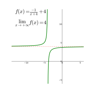
There are three basic rules for evaluating limits at infinity for a rational function

By noting that |x − p| represents a distance, the definition of a limit can be extended to functions of more than one variable.

Similar to the case in single variable, the value of f at (p, q) does not matter in this definition of limit.

We may consider taking the limit of just one variable, say, x → p, to obtain a single-variable function of y, namely

A sufficient condition of equality is given by the Moore-Osgood theorem, which requires the limit

Since this is also a finite-dimension vector-valued function, the limit theorem stated above also applies.

In fact, one can see that this definition is equivalent to that of the uniform limit of a multivariable function introduced in the previous section.

if the following property holds: This last part of the definition can also be phrased "there exists an open punctured neighbourhood U of p such that f(U ∩ Ω) ⊆ V".

Such a view is fundamental in the field of general topology, where limits and continuity at a point are defined in terms of special families of subsets, called filters, or generalized sequences known as nets.

Note that defining what it means for a sequence xn to converge to a requires the epsilon, delta method.

[23] On the other hand, Hrbacek writes that for the definitions to be valid for all hyperreal numbers they must implicitly be grounded in the ε-δ method, and claims that, from the pedagogical point of view, the hope that non-standard calculus could be done without ε-δ methods cannot be realized in full.

[24] Bŀaszczyk et al. detail the usefulness of microcontinuity in developing a transparent definition of uniform continuity, and characterize Hrbacek's criticism as a "dubious lament".

[25] At the 1908 international congress of mathematics F. Riesz introduced an alternate way defining limits and continuity in concept called "nearness".

The notion of the limit of a function is very closely related to the concept of continuity.

A function f is said to be continuous at c if it is both defined at c and its value at c equals the limit of f as x approaches c:

Additionally, the identity for division requires that the denominator on the right-hand side is non-zero (division by 0 is not defined), and the identity for exponentiation requires that the base is positive, or zero while the exponent is positive (finite).

In other cases the limit on the left may still exist, although the right-hand side, called an indeterminate form, does not allow one to determine the result.

This rule uses derivatives to find limits of indeterminate forms 0/0 or ±∞/∞, and only applies to such cases.