Matrix (mathematics)
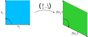
In geometry, matrices are widely used for specifying and representing geometric transformations (for example rotations) and coordinate changes.
There is no limit to the number of rows and columns, that a matrix (in the usual sense) can have as long as they are positive integers.
For example, The product cA of a number c (also called a scalar in this context) and a matrix A is computed by multiplying every entry of A by c:
In other words, matrix multiplication is not commutative, in marked contrast to (rational, real, or complex) numbers, whose product is independent of the order of the factors.
There are specifically adapted algorithms for, say, solving linear systems Ax = b for sparse matrices A, such as the conjugate gradient method.
[48] The original Dartmouth BASIC had built-in commands for matrix arithmetic on arrays from its second edition implementation in 1964.
As early as the 1970s, some engineering desktop computers such as the HP 9830 had ROM cartridges to add BASIC commands for matrices.
While most of these libraries require a professional level of coding, LAPACK can be accessed by higher-level (and user-friendly) bindings such as NumPy/SciPy, R, GNU Octave, MATLAB.
[50] Once this decomposition is calculated, linear systems can be solved more efficiently, by a simple technique called forward and back substitution.
More generally, and applicable to all matrices, the Jordan decomposition transforms a matrix into Jordan normal form, that is to say matrices whose only nonzero entries are the eigenvalues λ1 to λn of A, placed on the main diagonal and possibly entries equal to one directly above the main diagonal, as shown at the right.
As a first step of generalization, any field, that is, a set where addition, subtraction, multiplication, and division operations are defined and well-behaved, may be used instead of
More generally, any linear map f : V → W between finite-dimensional vector spaces can be described by a matrix A = (aij), after choosing bases v1, ..., vn of V, and w1, ..., wm of W (so n is the dimension of V and m is the dimension of W), which is such that In other words, column j of A expresses the image of vj in terms of the basis vectors wi of W; thus this relation uniquely determines the entries of the matrix A.
[63] More generally, the set of m×n matrices can be used to represent the R-linear maps between the free modules Rm and Rn for an arbitrary ring R with unity.
Infinite matrices can also be used to describe operators on Hilbert spaces, where convergence and continuity questions arise, which again results in certain constraints that must be imposed.
However, the explicit point of view of matrices tends to obfuscate the matter,[72] and the abstract and more powerful tools of functional analysis can be used instead.
[75] Text mining and automated thesaurus compilation makes use of document-term matrices such as tf-idf to track frequencies of certain words in several documents.
Chemistry makes use of matrices in various ways, particularly since the use of quantum theory to discuss molecular bonding and spectroscopy.
[95] For the three lightest quarks, there is a group-theoretical representation involving the special unitary group SU(3); for their calculations, physicists use a convenient matrix representation known as the Gell-Mann matrices, which are also used for the SU(3) gauge group that forms the basis of the modern description of strong nuclear interactions, quantum chromodynamics.
One particular example is the density matrix that characterizes the "mixed" state of a quantum system as a linear combination of elementary, "pure" eigenstates.
The best way to obtain solutions is to determine the system's eigenvectors, its normal modes, by diagonalizing the matrix equation.
The optical system, consisting of a combination of lenses and/or reflective elements, is simply described by the matrix resulting from the product of the components' matrices.
The Chinese text The Nine Chapters on the Mathematical Art written in the 10th–2nd century BCE is the first example of the use of array methods to solve simultaneous equations,[103] including the concept of determinants.
[105] The Dutch mathematician Jan de Witt represented transformations using arrays in his 1659 book Elements of Curves (1659).
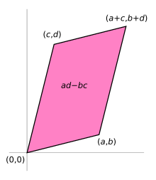
The term "matrix" (Latin for "womb", "dam" (non-human female animal kept for breeding), "source", "origin", "list", and "register", are derived from mater—mother[107]) was coined by James Joseph Sylvester in 1850,[108] who understood a matrix as an object giving rise to several determinants today called minors, that is to say, determinants of smaller matrices that derive from the original one by removing columns and rows.
In an 1851 paper, Sylvester explains:[109] I have in previous papers defined a "Matrix" as a rectangular array of terms, out of which different systems of determinants may be engendered from the womb of a common parent.Arthur Cayley published a treatise on geometric transformations using matrices that were not rotated versions of the coefficients being investigated as had previously been done.
Instead, he defined operations such as addition, subtraction, multiplication, and division as transformations of those matrices and showed the associative and distributive properties held.
[112] Number-theoretical problems led Gauss to relate coefficients of quadratic forms, that is, expressions such as x2 + xy − 2y2, and linear maps in three dimensions to matrices.
Kronecker's Vorlesungen über die Theorie der Determinanten[114] and Weierstrass' Zur Determinantentheorie,[115] both published in 1903, first treated determinants axiomatically, as opposed to previous more concrete approaches such as the mentioned formula of Cauchy.
The inception of matrix mechanics by Heisenberg, Born and Jordan led to studying matrices with infinitely many rows and columns.
Bertrand Russell and Alfred North Whitehead in their Principia Mathematica (1910–1913) use the word "matrix" in the context of their axiom of reducibility.