Maximum flow problem
The maximum value of an s-t flow (i.e., flow from source s to sink t) is equal to the minimum capacity of an s-t cut (i.e., cut severing s from t) in the network, as stated in the max-flow min-cut theorem.
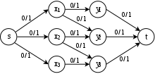
[4][5] In their 1955 paper,[4] Ford and Fulkerson wrote that the problem of Harris and Ross is formulated as follows (see[1] p. 5):Consider a rail network connecting two cities by way of a number of intermediate cities, where each link of the network has a number assigned to it representing its capacity.
Assuming a steady state condition, find a maximal flow from one given city to the other.In their book Flows in Networks,[5] in 1962, Ford and Fulkerson wrote:It was posed to the authors in the spring of 1955 by T. E. Harris, who, in conjunction with General F. S. Ross (Ret.
), had formulated a simplified model of railway traffic flow, and pinpointed this particular problem as the central one suggested by the model [11].where [11] refers to the 1955 secret report Fundamentals of a Method for Evaluating Rail net Capacities by Harris and Ross[3] (see[1] p. 5).
The algorithms of Sherman[6] and Kelner, Lee, Orecchia and Sidford,[7][8] respectively, find an approximately optimal maximum flow but only work in undirected graphs.
[9] In 2022 Li Chen, Rasmus Kyng, Yang P. Liu, Richard Peng, Maximilian Probst Gutenberg, and Sushant Sachdeva published an almost-linear time algorithm running in
[10][11] For the single-source shortest path (SSSP) problem with negative weights another particular case of minimum-cost flow problem an algorithm in almost-linear time has also been reported.
[12][13] Both algorithms were deemed best papers at the 2022 Symposium on Foundations of Computer Science.
The following table lists algorithms for solving the maximum flow problem.
, and a maximum cardinality matching can be found by taking those edges that have flow
, we are to find the minimum number of vertex-disjoint paths to cover each vertex in
vertices, the sum of the number of paths and edges in the cover is
It may be solved in polynomial time using a reduction to the maximum flow problem.
A team is eliminated if it has no chance to finish the season in the first place.
Schwartz[28] proposed a method which reduces this problem to maximum network flow.
One adds a game nodeij – which represents the number of plays between these two teams.
Finally, edges are made from team node i to the sink node t and the capacity of wk + rk – wi is set to prevent team i from winning more than wk + rk.
Let S be the set of all teams participating in the league and let In this method it is claimed team k is not eliminated if and only if a flow value of size r(S − {k}) exists in network G. In the mentioned article it is proved that this flow value is the maximum flow value from s to t. In the airline industry a major problem is the scheduling of the flight crews.
The airline scheduling problem can be considered as an application of extended maximum network flow.
One also adds the following edges to E: In the mentioned method, it is claimed and proved that finding a flow value of k in G between s and t is equal to finding a feasible schedule for flight set F with at most k crews.
[29] Another version of airline scheduling is finding the minimum needed crews to perform all the flights.
There exists a circulation that satisfies the demand if and only if : If there exists a circulation, looking at the max-flow solution would give the answer as to how much goods have to be sent on a particular road for satisfying the demands.
The problem can be extended by adding a lower bound on the flow on some edges.
[30] In their book, Kleinberg and Tardos present an algorithm for segmenting an image.
More precisely, the algorithm takes a bitmap as an input modelled as follows: ai ≥ 0 is the likelihood that pixel i belongs to the foreground, bi ≥ 0 in the likelihood that pixel i belongs to the background, and pij is the penalty if two adjacent pixels i and j are placed one in the foreground and the other in the background.
It is equivalent to minimize the quantity because We now construct the network whose nodes are the pixel, plus a source and a sink, see Figure on the right.
We connect the source to pixel i by an edge of weight ai.
Now, it remains to compute a minimum cut in that network (or equivalently a maximum flow).
In the minimum-cost flow problem, each edge (u,v) also has a cost-coefficient auv in addition to its capacity.
With negative constraints, the problem becomes strongly NP-hard even for simple networks.