Motion planning
A motion planning algorithm would take a description of these tasks as input, and produce the speed and turning commands sent to the robot's wheels.
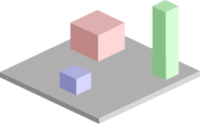
The robot and obstacle geometry is described in a 2D or 3D workspace, while the motion is represented as a path in (possibly higher-dimensional) configuration space.
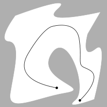
For example: The set of configurations that avoids collision with obstacles is called the free space Cfree.
Exact motion planning for high-dimensional systems under complex constraints is computationally intractable.
Potential-field algorithms are efficient, but fall prey to local minima (an exception is the harmonic potential fields).
Search is faster with coarser grids, but the algorithm will fail to find paths through narrow portions of Cfree.
Furthermore, the number of points on the grid grows exponentially in the configuration space dimension, which make them inappropriate for high-dimensional problems.
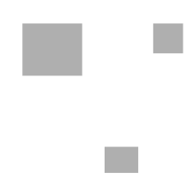
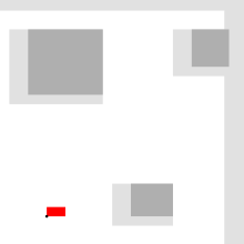
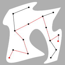
An illustration is provided by the three figures on the right where a hook with two degrees of freedom has to move from the left to the right, avoiding two horizontal small segments.
Nicolas Delanoue has shown that the decomposition with subpavings using interval analysis also makes it possible to characterize the topology of Cfree such as counting its number of connected components.
[2] Point robots among polygonal obstacles Translating objects among obstacles Finding the way out of a building Given a bundle of rays around the current position attributed with their length hitting a wall, the robot moves into the direction of the longest ray unless a door is identified.
One approach is to treat the robot's configuration as a point in a potential field that combines attraction to the goal, and repulsion from obstacles.
Given basic visibility conditions on Cfree, it has been proven that as the number of configurations N grows higher, the probability that the above algorithm finds a solution approaches 1 exponentially.
This is especially problematic, if there occur infinite sequences (that converge only in the limiting case) during a specific proving technique, since then, theoretically, the algorithm will never stop.
Intuitive "tricks" (often based on induction) are typically mistakenly thought to converge, which they do only for the infinite limit.
Planners based on a brute force approach are always complete, but are only realizable for finite and discrete setups.
In practice, the termination of the algorithm can always be guaranteed by using a counter, that allows only for a maximum number of iterations and then always stops with or without solution.
Completeness can only be provided by a very rigorous mathematical correctness proof (often aided by tools and graph based methods) and should only be done by specialized experts if the application includes safety content.
On the other hand, disproving completeness is easy, since one just needs to find one infinite loop or one wrong result returned.
Probabilistic completeness is the property that as more "work" is performed, the probability that the planner fails to find a path, if one exists, asymptotically approaches zero.
For practical applications, one usually uses this property, since it allows setting up the time-out for the watchdog based on an average convergence time.