In probability theory and statistics, the exponential distribution or negative exponential distribution is the probability distribution of the distance between events in a Poisson point process, i.e., a process in which events occur continuously and independently at a constant average rate; the distance parameter could be any meaningful mono-dimensional measure of the process, such as time between production errors, or length along a roll of fabric in the weaving manufacturing process.

The mean or expected value of an exponentially distributed random variable X with rate parameter λ is given by

The conditional value at risk (CVaR) also known as the expected shortfall or superquantile for Exp(λ) is derived as follows:[4]

In other words, it is the maximum entropy probability distribution for a random variate X which is greater than or equal to zero and for which E[X] is fixed.

[5] Let X1, ..., Xn be independent exponentially distributed random variables with rate parameters λ1, ..., λn.

independent and identically distributed exponential random variables with rate parameter λ.

The probability distribution function (PDF) of a sum of two independent random variables is the convolution of their individual PDFs.

are independent exponential random variables with respective rate parameters

The likelihood function for λ, given an independent and identically distributed sample x = (x1, ..., xn) drawn from the variable, is:

An approximate minimizer of mean squared error (see also: bias–variance tradeoff) can be found, assuming a sample size greater than two, with a correction factor to the MLE:

This determines the amount of information each independent sample of an exponential distribution carries about the unknown rate parameter

An exact 100(1 − α)% confidence interval for the rate parameter of an exponential distribution is given by:[13]

where χ2p,v is the 100(p) percentile of the chi squared distribution with v degrees of freedom, n is the number of observations and x-bar is the sample average.

The posterior distribution p can then be expressed in terms of the likelihood function defined above and a gamma prior:

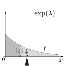
The exponential distribution occurs naturally when describing the lengths of the inter-arrival times in a homogeneous Poisson process.

In contrast, the exponential distribution describes the time for a continuous process to change state.

In real-world scenarios, the assumption of a constant rate (or probability per unit time) is rarely satisfied.

For example, the rate of incoming phone calls differs according to the time of day.

Similar caveats apply to the following examples which yield approximately exponentially distributed variables: Exponential variables can also be used to model situations where certain events occur with a constant probability per unit length, such as the distance between mutations on a DNA strand, or between roadkills on a given road.

In queuing theory, the service times of agents in a system (e.g. how long it takes for a bank teller etc.

Because of the memoryless property of this distribution, it is well-suited to model the constant hazard rate portion of the bathtub curve used in reliability theory.

It is also very convenient because it is so easy to add failure rates in a reliability model.

In physics, if you observe a gas at a fixed temperature and pressure in a uniform gravitational field, the heights of the various molecules also follow an approximate exponential distribution, known as the Barometric formula.

A common predictive distribution over future samples is the so-called plug-in distribution, formed by plugging a suitable estimate for the rate parameter λ into the exponential density function.

The Bayesian approach provides a predictive distribution which takes into account the uncertainty of the estimated parameter, although this may depend crucially on the choice of prior.

A predictive distribution free of the issues of choosing priors that arise under the subjective Bayesian approach is

Letting Δ(λ0||p) denote the Kullback–Leibler divergence between an exponential with rate parameter λ0 and a predictive distribution p it can be shown that

where the expectation is taken with respect to the exponential distribution with rate parameter λ0 ∈ (0, ∞), and ψ( · ) is the digamma function.

Other methods for generating exponential variates are discussed by Knuth[20] and Devroye.

[21] A fast method for generating a set of ready-ordered exponential variates without using a sorting routine is also available.