Standard RAID levels
In computer storage, the standard RAID levels comprise a basic set of RAID ("redundant array of independent disks" or "redundant array of inexpensive disks") configurations that employ the techniques of striping, mirroring, or parity to create large reliable data stores from multiple general-purpose computer hard disk drives (HDDs).
RAID levels and their associated data formats are standardized by the Storage Networking Industry Association (SNIA) in the Common RAID Disk Drive Format (DDF) standard.
[1] The numerical values only serve as identifiers and do not signify performance, reliability, generation, hierarchy, or any other metric.
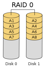
Since RAID 0 provides no fault tolerance or redundancy, the failure of one drive will cause the entire array to fail, due to data being striped across all disks.
[2][3] RAID 0 is normally used to increase performance, although it can also be used as a way to create a large logical volume out of two or more physical disks.
Once the stripe size is defined during the creation of a RAID 0 array, it needs to be maintained at all times.
As a result, RAID 0 is primarily used in applications that require high performance and are able to tolerate lower reliability, such as in scientific computing[5] or gaming.
[6] Some benchmarks of desktop applications show RAID 0 performance to be marginally better than a single drive.
[11][12] RAID 2, which is rarely used in practice, stripes data at the bit (rather than block) level, and uses a Hamming code for error correction.
The disks are synchronized by the controller to spin at the same angular orientation (they reach index at the same time[16]), so it generally cannot service multiple requests simultaneously.
With all hard disk drives implementing internal error correction, the complexity of an external Hamming code offered little advantage over parity so RAID 2 has been rarely implemented; it is the only original level of RAID that is not currently used.
[17][18] RAID 3, which is rarely used in practice, consists of byte-level striping with a dedicated parity disk.
One of the characteristics of RAID 3 is that it generally cannot service multiple requests simultaneously, which happens because any single block of data will, by definition, be spread across all members of the set and will reside in the same physical location on each disk.
This makes it suitable for applications that demand the highest transfer rates in long sequential reads and writes, for example uncompressed video editing.
Applications that make small reads and writes from random disk locations will get the worst performance out of this level.
[18] The requirement that all disks spin synchronously (in a lockstep) added design considerations that provided no significant advantages over other RAID levels.
[21] RAID 3 was usually implemented in hardware, and the performance issues were addressed by using large disk caches.
As a result of its layout, RAID 4 provides good performance of random reads, while the performance of random writes is low due to the need to write all parity data to a single disk,[22] unless the filesystem is RAID-4-aware and compensates for that.
An advantage of RAID 4 is that it can be quickly extended online, without parity recomputation, as long as the newly added disks are completely filled with 0-bytes.
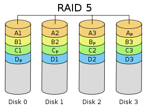
Upon failure of a single drive, subsequent reads can be calculated from the distributed parity such that no data is lost.
Although it will not be as efficient as a striping (RAID 0) setup, because parity must still be written, this is no longer a bottleneck.
This doubles CPU overhead for RAID-6 writes, versus single-parity RAID levels.
[citation needed] Reed Solomon coding also has the advantage of allowing all redundancy information to be contained within a given stripe.
[clarification needed] It is possible to support a far greater number of drives by choosing the parity function more carefully.
correspond to the stripes of data across hard drives encoded as field elements in this manner.
can be thought of as the action of a carefully chosen linear feedback shift register on the data chunk.
In the case of two lost data chunks, we can compute the recovery formulas algebraically.
In each case, array space efficiency is given as an expression in terms of the number of drives, n; this expression designates a fractional value between zero and one, representing the fraction of the sum of the drives' capacities that is available for use.
Different RAID configurations can also detect failure during so called data scrubbing.
The redundant information is used to reconstruct the missing data, rather than to identify the faulted drive.