Rotation matrix

For example, using the convention below, the matrix rotates points in the xy plane counterclockwise through an angle θ about the origin of a two-dimensional Cartesian coordinate system.

If any one of these is changed (such as rotating axes instead of vectors, a passive transformation), then the inverse of the example matrix should be used, which coincides with its transpose.

If a standard right-handed Cartesian coordinate system is used, with the x-axis to the right and the y-axis up, the rotation R(θ) is counterclockwise.

Such non-standard orientations are rarely used in mathematics but are common in 2D computer graphics, which often have the origin in the top left corner and the y-axis down the screen or page.

For example, the product represents a rotation whose yaw, pitch, and roll angles are α, β and γ, respectively.

Similarly, the product represents an extrinsic rotation whose (improper) Euler angles are α, β, γ, about axes x, y, z.

These matrices produce the desired effect only if they are used to premultiply column vectors, and (since in general matrix multiplication is not commutative) only if they are applied in the specified order (see Ambiguities for more details).

One way to determine the rotation axis is by showing that: Since (R − RT) is a skew-symmetric matrix, we can choose u such that The matrix–vector product becomes a cross product of a vector with itself, ensuring that the result is zero: Therefore, if then The magnitude of u computed this way is ‖u‖ = 2 sin θ, where θ is the angle of rotation.

A more direct method, however, is to simply calculate the trace: the sum of the diagonal elements of the rotation matrix.

In Euclidean geometry, a rotation is an example of an isometry, a transformation that moves points without changing the distances between them.

Now suppose (p1, ..., pn) are the coordinates of the vector p from the origin O to point P. Choose an orthonormal basis for our coordinates; then the squared distance to P, by Pythagoras, is which can be computed using the matrix multiplication A geometric rotation transforms lines to lines, and preserves ratios of distances between points.

From these properties it can be shown that a rotation is a linear transformation of the vectors, and thus can be written in matrix form, Qp.

In the three-dimensional case, the subspace consists of all vectors perpendicular to the rotation axis (the invariant direction, with eigenvalue 1).

To solve for θ it is not enough to look at a alone or b alone; we must consider both together to place the angle in the correct quadrant, using a two-argument arctangent function.

We can zero them by extending the same idea of stepping through the columns with a series of rotations in a fixed sequence of planes.

Thus we find many different conventions employed when three-dimensional rotations are parameterized for physics, or medicine, or chemistry, or other disciplines.

One reason for the large number of options is that, as noted previously, rotations in three dimensions (and higher) do not commute.

A direction in (n + 1)-dimensional space will be a unit magnitude vector, which we may consider a point on a generalized sphere, Sn.

In three dimensions, for example, we have (Cayley 1846) If we condense the skew entries into a vector, (x,y,z), then we produce a 90° rotation around the x-axis for (1, 0, 0), around the y-axis for (0, 1, 0), and around the z-axis for (0, 0, 1).

The BCH formula provides an explicit expression for Z = log(eXeY) in terms of a series expansion of nested commutators of X and Y.

We can, in fact, obtain all four magnitudes using sums and square roots, and choose consistent signs using the skew-symmetric part of the off-diagonal entries: Alternatively, use a single square root and division This is numerically stable so long as the trace, t, is not negative; otherwise, we risk dividing by (nearly) zero.

If the n × n matrix M is nonsingular, its columns are linearly independent vectors; thus the Gram–Schmidt process can adjust them to be an orthonormal basis.

Stated in terms of numerical linear algebra, we convert M to an orthogonal matrix, Q, using QR decomposition.

Including constraints, we seek to minimize Taking the derivative with respect to Qxx, Qxy, Qyx, Qyy in turn, we assemble a matrix.

To efficiently construct a rotation matrix Q from an angle θ and a unit axis u, we can take advantage of symmetry and skew-symmetry within the entries.

Suppose the three angles are θ1, θ2, θ3; physics and chemistry may interpret these as while aircraft dynamics may use One systematic approach begins with choosing the rightmost axis.

For example, suppose we use the zyz convention above; then we have the following equivalent pairs: Angles for any order can be found using a concise common routine (Herter & Lott 1993; Shoemake 1994).

The singularities are avoided when considering and manipulating the rotation matrix as orthonormal row vectors (in 3D applications often named the right-vector, up-vector and out-vector) instead of as angles.

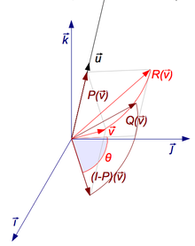
In some instances it is interesting to describe a rotation by specifying how a vector is mapped into another through the shortest path (smallest angle).

León, Massé & Rivest (2006) show how to use the Cayley transform to generate and test matrices according to this criterion.