Without loss of generality, we can consider only centered profiles, which peak at zero.

The Voigt profile is then where x is the shift from the line center,

is the centered Lorentzian profile: The defining integral can be evaluated as: where Re[w(z)] is the real part of the Faddeeva function evaluated for In the limiting cases of

Voigt profiles are common in many branches of spectroscopy and diffraction.

The Lorentzian profile has no moments (other than the zeroth), and so the moment-generating function for the Cauchy distribution is not defined.

Using the above definition for z , the cumulative distribution function (CDF) can be found as follows: Substituting the definition of the Faddeeva function (scaled complex error function) yields for the indefinite integral: which may be solved to yield where

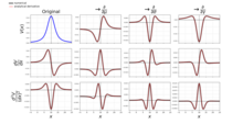
, the first and second derivatives can be expressed in terms of the Faddeeva function as and respectively.

Often, one or multiple Voigt profiles and/or their respective derivatives need to be fitted to a measured signal by means of non-linear least squares, e.g., in spectroscopy.

Then, further partial derivatives can be utilised to accelerate computations.

Instead of approximating the Jacobian matrix with respect to the parameters

with the aid of finite differences, the corresponding analytical expressions can be applied.

play a relatively similar role in the calculation of

All these derivatives involve only simple operations (multiplications and additions) because the computationally expensive

Such a reuse of previous calculations allows for a derivation at minimum costs.

This is not the case for finite difference gradient approximation as it requires the evaluation of

[2] It is obtained from a truncated power series expansion of the exact line broadening function.

In its most computationally efficient form, the Tepper-García function can be expressed as where

Thus the line broadening function can be viewed, to first order, as a pure Gaussian function plus a correction factor that depends linearly on the microscopic properties of the absorbing medium (encoded in

); however, as a result of the early truncation in the series expansion, the error in the approximation is still of order

This approximation has a relative accuracy of over the full wavelength range of

It is widely used in the field of quasar absorption line analysis.

[3] The pseudo-Voigt profile (or pseudo-Voigt function) is an approximation of the Voigt profile V(x) using a linear combination of a Gaussian curve G(x) and a Lorentzian curve L(x) instead of their convolution.

The pseudo-Voigt function is often used for calculations of experimental spectral line shapes.

The mathematical definition of the normalized pseudo-Voigt profile is given by

is a function of full width at half maximum (FWHM) parameter.

) Full width at half maximum (FWHM) parameters.

The FWHM of the Gaussian profile is The FWHM of the Lorentzian profile is An approximate relation (accurate to within about 1.2%) between the widths of the Voigt, Gaussian, and Lorentzian profiles is:[10] By construction, this expression is exact for a pure Gaussian or Lorentzian.

A better approximation with an accuracy of 0.02% is given by [11] (originally found by Kielkopf[12]) Again, this expression is exact for a pure Gaussian or Lorentzian.

In the same publication,[11] a slightly more precise (within 0.012%), yet significantly more complicated expression can be found.

The asymmetry pseudo-Voigt (Martinelli) function resembles a split normal distribution by having different widths on each side of the peak position.