Autonomous system (mathematics)
In mathematics, an autonomous system or autonomous differential equation is a system of ordinary differential equations which does not explicitly depend on the independent variable.
When the variable is time, they are also called time-invariant systems.
Many laws in physics, where the independent variable is usually assumed to be time, are expressed as autonomous systems because it is assumed the laws of nature which hold now are identical to those for any point in the past or future.
where x takes values in n-dimensional Euclidean space; t is often interpreted as time.
It is distinguished from systems of differential equations of the form
Solutions are invariant under horizontal translations: Let
be a unique solution of the initial value problem for an autonomous system
For the initial condition, the verification is trivial,
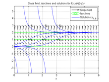
To plot the slope field and isocline for this equation, one can use the following code in GNU Octave/MATLAB One can observe from the plot that the function
Solving the equation symbolically in MATLAB, by running obtains two equilibrium solutions,
, and a third solution involving an unknown constant
Picking up some specific values for the initial condition, one can add the plot of several solutions Autonomous systems can be analyzed qualitatively using the phase space; in the one-variable case, this is the phase line.
The following techniques apply to one-dimensional autonomous differential equations.
is separable, so it can be solved by rearranging it into the integral form
which is a first order equation containing no reference to the independent variable
[3] These types of equations are very common in classical mechanics because they are always Hamiltonian systems.
which follows from the chain rule, barring any issues due to division by zero.
By inverting both sides of a first order autonomous system, one can immediately integrate with respect to
which is another way to view the separation of variables technique.
To reemphasize: what's been accomplished is that the second derivative with respect to
The greatest potential problem is inability to simplify the integrals, which implies difficulty or impossibility in evaluating the integration constants.
Using the above approach, the technique can extend to the more general equation
This will work since the second derivative can be written in a form involving a power of
There is no analogous method for solving third- or higher-order autonomous equations.
Such equations can only be solved exactly if they happen to have some other simplifying property, for instance linearity or dependence of the right side of the equation on the dependent variable only[4][5] (i.e., not its derivatives).
This should not be surprising, considering that nonlinear autonomous systems in three dimensions can produce truly chaotic behavior such as the Lorenz attractor and the Rössler attractor.
Likewise, general non-autonomous equations of second order are unsolvable explicitly, since these can also be chaotic, as in a periodically forced pendulum.
[7] For non-linear autonomous ODEs it is possible under some conditions to develop solutions of finite duration,[8] meaning here that from its own dynamics, the system will reach the value zero at an ending time and stay there in zero forever after.
These finite-duration solutions cannot be analytical functions on the whole real line, and because they will be non-Lipschitz functions at the ending time, they don't stand[clarification needed] uniqueness of solutions of Lipschitz differential equations.
As example, the equation: Admits the finite duration solution: