Euler method
In mathematics and computational science, the Euler method (also called the forward Euler method) is a first-order numerical procedure for solving ordinary differential equations (ODEs) with a given initial value.
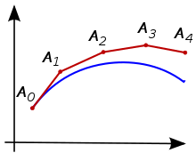
Consider the problem of calculating the shape of an unknown curve which starts at a given point and satisfies a given differential equation.
The idea is that while the curve is initially unknown, its starting point, which we denote by
, we implement the following formula until we reach the approximation of the solution to the ODE at the desired time: These first-order systems can be handled by Euler's method or, in fact, by any other scheme for first-order systems.
[4] Given the initial value problem we would like to use the Euler method to approximate
We have By doing the above step, we have found the slope of the line that is tangent to the solution curve at the point
Due to the repetitive nature of this algorithm, it can be helpful to organize computations in a chart form, as seen below, to avoid making errors.
Although the approximation of the Euler method was not very precise in this specific case, particularly due to a large value step size
As suggested in the introduction, the Euler method is more accurate if the step size
The table below shows the result with different step sizes.
The error recorded in the last column of the table is the difference between the exact solution at
In the bottom of the table, the step size is half the step size in the previous row, and the error is also approximately half the error in the previous row.
This is true in general, also for other equations; see the section Global truncation error for more details.
This large number of steps entails a high computational cost.
If this is substituted in the Taylor expansion and the quadratic and higher-order terms are ignored, the Euler method arises.
and apply the fundamental theorem of calculus to get: Now approximate the integral by the left-hand rectangle method (with only one rectangle): Combining both equations, one finds again the Euler method.
This line of thought can be continued to arrive at various linear multistep methods.
The numerical solution is given by For the exact solution, we use the Taylor expansion mentioned in the section Derivation above: The local truncation error (LTE) introduced by the Euler method is given by the difference between these equations: This result is valid if
A slightly different formulation for the local truncation error can be obtained by using the Lagrange form for the remainder term in Taylor's theorem.
can be replaced by an expression involving the right-hand side of the differential equation.
is Lipschitz continuous in its second argument, then the global truncation error (denoted as
[16] What is important is that it shows that the global truncation error is (approximately) proportional to
The Euler method can also be numerically unstable, especially for stiff equations, meaning that the numerical solution grows very large for equations where the exact solution does not.
, then the numerical solution is qualitatively wrong: It oscillates and grows (see the figure).
— means that the Euler method is not often used, except as a simple example of numerical integration[citation needed].
Frequently models of physical systems contain terms representing fast-decaying elements (i.e. with large negative exponential arguments).
Even when these are not of interest in the overall solution, the instability they can induce means that an exceptionally small timestep would be required if the Euler method is used.
Most of the effect of rounding error can be easily avoided if compensated summation is used in the formula for the Euler method.
on both sides, so when applying the backward Euler method we have to solve an equation.
There are other modifications which uses techniques from compressive sensing to minimize memory usage[21] In the film Hidden Figures, Katherine Johnson resorts to the Euler method in calculating the re-entry of astronaut John Glenn from Earth orbit.