The beta distribution has been applied to model the behavior of random variables limited to intervals of finite length in a wide variety of disciplines.

Denoting by αPosterior and βPosterior the shape parameters of the posterior beta distribution resulting from applying Bayes theorem to a binomial likelihood function and a prior probability, the interpretation of the addition of both shape parameters to be sample size = ν = α·Posterior + β·Posterior is only correct for the Haldane prior probability Beta(0,0).

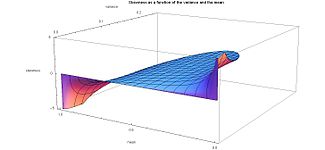
Excess kurtosis reaches the minimum possible value (for any distribution) when the probability density function has two spikes at each end: it is bi-"peaky" with nothing in between them.

Alternatively, the excess kurtosis can also be expressed in terms of just the following two parameters: the square of the skewness, and the sample size ν as follows: From this last expression, one can obtain the same limits published over a century ago by Karl Pearson[21] for the beta distribution (see section below titled "Kurtosis bounded by the square of the skewness").

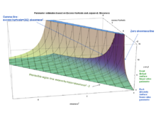
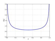
The lower boundary line (excess kurtosis + 2 − skewness2 = 0) is produced by skewed "U-shaped" beta distributions with both values of shape parameters α and β close to zero.

The boundary for this "impossible region" is determined by (symmetric or skewed) bimodal U-shaped distributions for which the parameters α and β approach zero and hence all the probability density is concentrated at the ends: x = 0, 1 with practically nothing in between them.

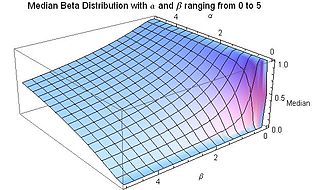
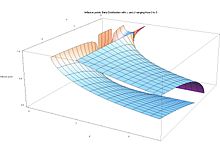
The beta density function can take a wide variety of different shapes depending on the values of the two parameters α and β.

The ability of the beta distribution to take this great diversity of shapes (using only two parameters) is partly responsible for finding wide application for modeling actual measurements: The density function is skewed.

If X1, ..., XN are independent random variables each having a beta distribution, the joint log likelihood function for N iid observations is: Finding the maximum with respect to a shape parameter involves taking the partial derivative with respect to the shape parameter and setting the expression equal to zero yielding the maximum likelihood estimator of the shape parameters: where: since the digamma function denoted ψ(α) is defined as the logarithmic derivative of the gamma function:[18] To ensure that the values with zero tangent slope are indeed a maximum (instead of a saddle-point or a minimum) one has to also satisfy the condition that the curvature is negative.

This amounts to satisfying that the second partial derivative with respect to the shape parameters is negative using the previous equations, this is equivalent to: where the trigamma function, denoted ψ1(α), is the second of the polygamma functions, and is defined as the derivative of the digamma function: These conditions are equivalent to stating that the variances of the logarithmically transformed variables are positive, since: Therefore, the condition of negative curvature at a maximum is equivalent to the statements: Alternatively, the condition of negative curvature at a maximum is also equivalent to stating that the following logarithmic derivatives of the geometric means GX and G(1−X) are positive, since: While these slopes are indeed positive, the other slopes are negative: The slopes of the mean and the median with respect to α and β display similar sign behavior.

can be obtained in terms of the inverse[49] digamma function of the right hand side of this equation: In particular, if one of the shape parameters has a value of unity, for example for

N.L.Johnson and S.Kotz[1] ignore the equations for the harmonic means and instead suggest "If a and c are unknown, and maximum likelihood estimators of a, c, α and β are required, the above procedure (for the two unknown parameter case, with X transformed as X = (Y − a)/(c − a)) can be repeated using a succession of trial values of a and c, until the pair (a, c) for which maximum likelihood (given a and c) is as great as possible, is attained" (where, for the purpose of clarity, their notation for the parameters has been translated into the present notation).

The partial derivative with respect to the (unknown, and to be estimated) parameter α of the log likelihood function is called the score.

If the log likelihood function is twice differentiable with respect to the parameter α, and under certain regularity conditions,[50] then the Fisher information may also be written as follows (which is often a more convenient form for calculation purposes): Thus, the Fisher information is the negative of the expectation of the second derivative with respect to the parameter α of the log likelihood function.

For X1, ..., XN independent random variables each having a beta distribution parametrized with shape parameters α and β, the joint log likelihood function for N iid observations is: therefore the joint log likelihood function per N iid observations is For the two parameter case, the Fisher information has 4 components: 2 diagonal and 2 off-diagonal.

A classic application of the beta distribution is the rule of succession, introduced in the 18th century by Pierre-Simon Laplace[55] in the course of treating the sunrise problem.

These problems with Laplace's rule of succession motivated Haldane, Perks, Jeffreys and others to search for other forms of prior probability (see the next § Bayesian inference).

Harold Jeffreys[59][65] proposed to use an uninformative prior probability measure that should be invariant under reparameterization: proportional to the square root of the determinant of Fisher's information matrix.

They cannot obtain a closed-form expression for their reference prior, but numerical calculations show it to be nearly perfectly fitted by the (proper) prior where θ is the vertex variable for the asymmetric triangular distribution with support [0, 1] (corresponding to the following parameter values in Wikipedia's article on the triangular distribution: vertex c = θ, left end a = 0,and right end b = 1).

Berger et al. also give a heuristic argument that Beta(1/2,1/2) could indeed be the exact Berger–Bernardo–Sun reference prior for the asymmetric triangular distribution.

If samples are drawn from the population of a random variable X that result in s successes and f failures in n Bernoulli trials n = s + f, then the likelihood function for parameters s and f given x = p (the notation x = p in the expressions below will emphasize that the domain x stands for the value of the parameter p in the binomial distribution), is the following binomial distribution: If beliefs about prior probability information are reasonably well approximated by a beta distribution with parameters α Prior and β Prior, then: According to Bayes' theorem for a continuous event space, the posterior probability density is given by the product of the prior probability and the likelihood function (given the evidence s and f = n − s), normalized so that the area under the curve equals one, as follows: The binomial coefficient appears both in the numerator and the denominator of the posterior probability, and it does not depend on the integration variable x, hence it cancels out, and it is irrelevant to the final result.

Similarly the normalizing factor for the prior probability, the beta function B(αPrior,βPrior) cancels out and it is immaterial to the final result.

However, this happens only in degenerate cases (in this example n = 3 and hence s = 3/4 < 1, a degenerate value because s should be greater than unity in order for the posterior of the Haldane prior to have a mode located between the ends, and because s = 3/4 is not an integer number, hence it violates the initial assumption of a binomial distribution for the likelihood) and it is not an issue in generic cases of reasonable sample size (such that the condition 1 < s < n − 1, necessary for a mode to exist between both ends, is fulfilled).

K. Pearson wrote: "Yet the only supposition that we appear to have made is this: that, knowing nothing of nature, routine and anomy (from the Greek ανομία, namely: a- "without", and nomos "law") are to be considered as equally likely to occur.

In our ignorance we ought to consider before experience that nature may consist of all routines, all anomies (normlessness), or a mixture of the two in any proportion whatever, and that all such are equally probable.

In project management, shorthand computations are widely used to estimate the mean and standard deviation of the beta distribution:[39] where a is the minimum, c is the maximum, and b is the most likely value (the mode for α > 1 and β > 1).

William P. Elderton in his 1906 monograph "Frequency curves and correlation"[42] further analyzes the beta distribution as Pearson's Type I distribution, including a full discussion of the method of moments for the four parameter case, and diagrams of (what Elderton describes as) U-shaped, J-shaped, twisted J-shaped, "cocked-hat" shapes, horizontal and angled straight-line cases.

Also according to Bowman and Shenton, "the case of a Type I (beta distribution) model being the center of the controversy was pure serendipity.

The long running public conflict of Fisher with Karl Pearson can be followed in a number of articles in prestigious journals.

N.L.Johnson and S.Kotz, in their comprehensive and very informative monograph[83] on leading historical personalities in statistical sciences credit Corrado Gini[84] as "an early Bayesian...who dealt with the problem of eliciting the parameters of an initial Beta distribution, by singling out techniques which anticipated the advent of the so-called empirical Bayes approach."