Butterfly diagram
In the context of fast Fourier transform algorithms, a butterfly is a portion of the computation that combines the results of smaller discrete Fourier transforms (DFTs) into a larger DFT, or vice versa (breaking a larger DFT up into subtransforms).
[2][3] The same structure can also be found in the Viterbi algorithm, used for finding the most likely sequence of hidden states.
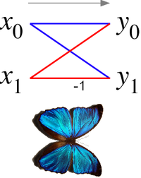
In the case of the radix-2 Cooley–Tukey algorithm, the butterfly is simply a DFT of size-2 that takes two inputs (x0, x1) (corresponding outputs of the two sub-transforms) and gives two outputs (y0, y1) by the formula (not including twiddle factors): If one draws the data-flow diagram for this pair of operations, the (x0, x1) to (y0, y1) lines cross and resemble the wings of a butterfly, hence the name (see also the illustration at right).
More specifically, a radix-2 decimation-in-time FFT algorithm on n = 2 p inputs with respect to a primitive n-th root of unity
Whereas the corresponding inverse transform can mathematically be performed by replacing ω with ω−1 (and possibly multiplying by an overall scale factor, depending on the normalization convention), one may also directly invert the butterflies: corresponding to a decimation-in-frequency FFT algorithm.