Calibration curve
In analytical chemistry, a calibration curve, also known as a standard curve, is a general method for determining the concentration of a substance in an unknown sample by comparing the unknown to a set of standard samples of known concentration.
In more general use, a calibration curve is a curve or table for a measuring instrument which measures some parameter indirectly, giving values for the desired quantity as a function of values of sensor output.
[2] Such a curve is typically used when an instrument uses a sensor whose calibration varies from one sample to another, or changes with time or use; if sensor output is consistent the instrument would be marked directly in terms of the measured unit.
The concentrations of the standards must lie within the working range of the technique (instrumentation) they are using.
[3] Analyzing each of these standards using the chosen technique will produce a series of measurements.
For most analyses a plot of instrument response vs. concentration will show a linear relationship.
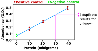
The operator can measure the response of the unknown and, using the calibration curve, can interpolate to find the concentration of analyte.
The data – the concentrations of the analyte and the instrument response for each standard – can be fit to a straight line, using linear regression analysis.
For instance, chromium (III) might be measured using a chemiluminescence method, in an instrument that contains a photomultiplier tube (PMT) as the detector.
The reagent Coomassie brilliant blue turns blue when it binds to arginine and aromatic amino acids present in proteins, thus increasing the absorbance of the sample.
The corresponding value on the X-axis is the concentration of substance in the unknown sample.
First, the calibration curve provides a reliable way to calculate the uncertainty of the concentration calculated from the calibration curve (using the statistics of the least squares line fit to the data).
(Instrumental response is usually highly dependent on the condition of the analyte, solvents used and impurities it may contain; it could also be affected by external factors such as pressure and temperature.)
Many theoretical relationships, such as fluorescence, require the determination of an instrumental constant anyway, by analysis of one or more reference standards; a calibration curve is a convenient extension of this approach.
The calibration curve for a particular analyte in a particular (type of) sample provides the empirical relationship needed for those particular measurements.
Some analytes – e.g., particular proteins – are extremely difficult to obtain pure in sufficient quantity.
Other analytes are often in complex matrices, e.g., heavy metals in pond water.