Chaotic mixing

A fluid flow can be considered as a dynamical system, that is a set of ordinary differential equations that determines the evolution of a Lagrangian trajectory.

Thus, a spot of dyed fluid to be mixed can only explore the region bounded by the most external and internal streamline, on which it is lying at the initial time.

For 2-D unstationary (time-dependent) flows, instantaneous closed streamlines and Lagrangian trajectories do not coincide any more.

A famous example is the blinking vortex flow introduced by Aref,[4] where two fixed rod-like agitators are alternately rotated inside the fluid.

Switching periodically the active (rotating) agitator introduces a time-dependency in the flow, which results in chaotic advection.

Lagrangian trajectories can therefore escape from closed streamlines, and visit a large fraction of the fluid domain.

is the ith principal component of the matrix H. If we start with a set of orthonormal initial error vectors,

The action of the system maps an infinitesimal sphere of inititial points to an ellipsoid whose major axis is given by the

In a chaotic system, we call the Lyapunov exponent the asymptotic value of the greatest eigenvalue of H: If there is any significant difference between the Lyapunov exponents then as an error vector evolves forward in time, any displacement in the direction of largest growth will tend to be magnified.

This can be understood very simply and intuitively by considering two nearby points: since the difference in tracer concentration will be fixed, the only source of variation in the gradients between them will be their separation.

A Poincaré section is built by starting from a few different initial conditions and plotting the corresponding iterates.

As an example, the figure presented here (left part) depicts the Poincaré section obtained when one applies periodically a figure-eight-like movement to a circular mixing rod.

Generally speaking, changing the geometry of the flow can modify the presence or absence of islands.

With a larger rod (right part of the figure), particles can escape from these loops and islands do not exist any more, resulting in better mixing.

With a Poincaré section, the mixing quality of a flow can be analyzed by distinguishing between chaotic and elliptic regions.

This is a crude measure of the mixing process, however, since the stretching properties cannot be inferred from this mapping method.

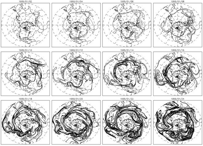
Through a continual process of stretching and folding, much like in a "baker's map," tracers advected in chaotic flows will develop into complex fractals.

Exponential growth ensures that the contour, in the limit of very long time integration, becomes fractal.

Fractals composed of a single curve are infinitely long and when formed iteratively, have an exponential growth rate, just like an advected contour.

The figure below shows the fractal dimension of an advected contour as a function of time, measured in four different ways.

A good method of measuring the fractal dimension of an advected contour is the uncertainty exponent.

The width of a dye filament decreases exponentially with time, until an equilibrium scale is reached, at which the effect of diffusion starts to be significant.

The resolution of the advection–diffusion equation shows that after the mixing time of a filament, the decrease of the concentration fluctuation due to diffusion is exponential, resulting in fast homogenization with the surrounding fluid.

The birth of the theory of chaotic advection is usually traced back to a 1984 paper[4] by Hassan Aref.

In this work, Aref studied the mixing induced by two vortices switched alternately on and off inside an inviscid fluid.

This seminal work had been made possible by earlier developments in the fields of dynamical Systems and fluid mechanics in the previous decades.

Vladimir Arnold[8] and Michel Hénon[9] had already noticed that the trajectories advected by area-preserving three-dimensional flows could be chaotic.

However, the practical interest of chaotic advection for fluid mixing applications remained unnoticed until the work of Aref in the 80's.

Since then, the whole toolkit of dynamical systems and chaos theory has been used to characterize fluid mixing by chaotic advection.

[1] Recent work has for example employed topological methods to characterize the stretching of fluid particles.