Chebyshev filter
The transfer function must be stable, so that its poles are those of the gain that have negative real parts and therefore lie in the left half plane of complex frequency space.
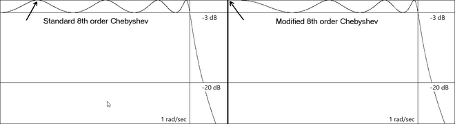
Even order Chebyshev filters implemented with passive elements, typically inductors, capacitors, and transmission lines, with terminations of equal value on each side cannot be implemented with the traditional Chebyshev transfer function without the use of coupled coils, which may not be desirable or feasible, particularly at the higher frequencies.
If it is not feasible to design the filter with one of the terminations increased or decreased to accommodate the pass band S12, then the Chebyshev transfer function must be modified so as to move the lowest even order reflection zero to
[5] The needed modification involves mapping each pole of the Chebyshev transfer function in a manner that maps the lowest frequency reflection zero to zero and the remaining poles as needed to maintain the equi-ripple pass band.
The LC element value formulas in the Cauer topology are not applicable to the even order modified Chebyshev transfer function, and cannot be used.
Even order modifications and finite stop band transmission zeros will introduce error that the equations do not account for.
However, many applications such as diplexers and triplexers,[5] require a cutoff attenuation of -3.0103 dB in order to obtain the needed reflections.
The scaling factor may be determined by direct algebraic manipulation of the defining Chebyshev filter function,
This makes the even order adjustment arithmetic slightly simpler, since frequency can be treated as a real variable, in this case
The gain and the group delay for a fifth-order type II Chebyshev filter with ε=0.1 are plotted in the graph on the left.
The equations is identical to that used for Chebyshev filter minimum order, with a slightly different variable definitions.
th-order Chebyshev prototype filter may be calculated from the following equations:[8] G1, Gk are the capacitor or inductor element values.
For example, or Note that when G1 is a shunt capacitor or series inductor, G0 corresponds to the input resistance or conductance, respectively.
As with most analog filters, the Chebyshev may be converted to a digital (discrete-time) recursive form via the bilinear transform.
The algorithm is extremely efficient if the Binomial coefficients are implemented from a look-up table of pre-calculated values.
Even order finite transmission zero Chebyshev filters have the same limitation as the all-pole case in that they cannot be constructed using equally terminated passive networks.
This movement may be significantly mitigated by propositioning the transmission zeros with the inverse of the even order modification using the lowest Chebyshev node,
The filter will also be asymmetric if finite transmission zeros are not place symmetrically about the geometric center frequency, which in this case is
Real and complex quadruplet transmission zeros may also be created using this technique and are useful to modify the group delay response, just as in the low pass case.
Constricting the equi-ripple to a defined percentage of the pass band creates a more efficient design, reducing the size of the filter and potentially eliminating one or two components, which is useful in maximizing board space efficiency and minimizing production costs for mass produced items.
Added reflection zeros introduces a noticeable error in the pass band that is likely to be objectionable.
This error may be removed quickly and accurately by repositioning the finite reflection zeros with the use of Newton's method for systems of equations.
Positioning the reflection zeros with Newton's method requires three pieces of information: Since the Chebyshev characteristic equations,
axis (required for passive element implementation), the locations of the pass band ripple minima may be obtained by factoring the numerator of the derivative of
from the pass band zero derivative frequencies by computing the positive real or imaginary values of the roots of
Standard low pass Inverse Chebyshev filter design creates an equi-ripple stop band beginning from a normalized value of 1 rad/sec to
Constricting the equi-ripple to a defined percentage of the stop band creates a more efficient design, reducing the size of the filter and potentially eliminating one or two components, which is useful in maximizing board space efficiency and minimizing production costs for mass produced items.
Below are the |S11| and |S12| scattering parameters for a 7 pole constricted ripple Inverse Chebyshev filter with 3dB cut-off attenuation.
The constricted ripple example above is intentionally kept simple by keeping the cut-off attenuation equal to the pass band ripple attenuation, omitting optional transmission zeros, and using an odd order that does not potentially require even order modification.
However, non-standard cutoff attenuations may be accommodated by calculating the target values in step 5 to be offset from the required 1 that exists at the cut-off frequency of


| Step 1: |
|---|
| 7 pole 55% constricted ripple pass band for |
| 1dB equi-ripple pass band |
| Linear frequency scale |


| Step 2: |
|---|
| 7 pole 55% constricted ripple pass band for |
| 1dB equi-ripple pass band |
| Linear frequency scale |

| Step final: |
|---|
| 7 pole 55% constricted ripple pass band for |
| 1dB equi-ripple pass band |
| Linear frequency scale |


| Step final: |
|---|
| 8 pole 55% constricted ripple pass band for |
| 20dB S11 equi-ripple pass band |
| finite transmission zero at 1.1 rad/sec |
| non-standard S12 cut-off attenuation at 20dB |
| Geometric frequency scale |