Butterworth filter
It was first described in 1930 by the British engineer and physicist Stephen Butterworth in his paper entitled "On the Theory of Filter Amplifiers".
Butterworth had a reputation for solving very complex mathematical problems thought to be 'impossible'.
Butterworth stated that: "An ideal electrical filter should not only completely reject the unwanted frequencies but should also have uniform sensitivity for the wanted frequencies".Such an ideal filter cannot be achieved, but Butterworth showed that successively closer approximations were obtained with increasing numbers of filter elements of the right values.
At the time, filters generated substantial ripple in the passband, and the choice of component values was highly interactive.
Its cutoff frequency (the half-power point of approximately −3 dB or a voltage gain of 1/√2 ≈ 0.7071) is normalized to 𝜔 = 1 radian per second.
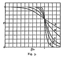
His plot of the frequency response of 2-, 4-, 6-, 8-, and 10-pole filters is shown as A, B, C, D, and E in his original graph.
Butterworth solved the equations for two-pole and four-pole filters, showing how the latter could be cascaded when separated by vacuum tube amplifiers and so enabling the construction of higher-order filters despite inductor losses.
In 1930, low-loss core materials such as molypermalloy had not been discovered and air-cored audio inductors were rather lossy.
Butterworth discovered that it was possible to adjust the component values of the filter to compensate for the winding resistance of the inductors.
He used coil forms of 1.25″ diameter and 3″ length with plug-in terminals.
Associated capacitors and resistors were contained inside the wound coil form.
The frequency response of the Butterworth filter is maximally flat (i.e., has no ripples) in the passband and rolls off towards zero in the stopband.
[2] When viewed on a logarithmic Bode plot, the response slopes off linearly towards negative infinity.
, unlike other filter types that have non-monotonic ripple in the passband and/or the stopband.
A transfer function of a third-order low-pass Butterworth filter design shown in the figure on the right looks like this: A simple example of a Butterworth filter is the third-order low-pass design shown in the figure on the right, with
The function is defined by the three poles in the left half of the complex frequency plane.
th-order Butterworth low-pass filter is given in terms of the transfer function
Factors of Butterworth polynomials of order 1 through 6 are shown in the following table (Exact).
are: The normalized Butterworth polynomials can be used to determine the transfer function for any low-pass filter cut-off frequency
, the derivative of the gain with respect to frequency can be shown to be which is monotonically decreasing for all
If the requirement to be monotonic is limited to the passband only and ripples are allowed in the stopband, then it is possible to design a filter of the same order, such as the inverse Chebyshev filter, that is flatter in the passband than the "maximally flat" Butterworth.
dB/octave (the factor of 20 is used because the power is proportional to the square of the voltage gain; see 20 log rule.)
The Cauer topology uses passive components (shunt capacitors and series inductors) to implement a linear analog filter.
The Butterworth filter having a given transfer function can be realised using a Cauer 1-form.
The k-th element is given by[10] The filter may start with a series inductor if desired, in which case the Lk are k odd and the Ck are k even.
These formulae may usefully be combined by making both Lk and Ck equal to gk.
That is, gk is the immittance divided by s. These formulae apply to a doubly terminated filter (that is, the source and load impedance are both equal to unity) with ωc = 1.
[3] The Sallen–Key topology uses active and passive components (noninverting buffers, usually op amps, resistors, and capacitors) to implement a linear analog filter.
is odd), this must be implemented separately, usually as an RC circuit, and cascaded with the active stages.
For the second-order Sallen–Key circuit shown to the right the transfer function is given by We wish the denominator to be one of the quadratic terms in a Butterworth polynomial.