Control theory
The objective is to develop a model or algorithm governing the application of system inputs to drive the system to a desired state, while minimizing any delay, overshoot, or steady-state error and ensuring a level of control stability; often with the aim to achieve a degree of optimality.
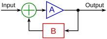
The difference between actual and desired value of the process variable, called the error signal, or SP-PV error, is applied as feedback to generate a control action to bring the controlled process variable to the same value as the set point.
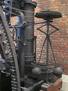
Control theory dates from the 19th century, when the theoretical basis for the operation of governors was first described by James Clerk Maxwell.
[5] Maxwell described and analyzed the phenomenon of self-oscillation, in which lags in the system may lead to overcompensation and unstable behavior.
In contemporary vessels, they may be gyroscopically controlled active fins, which have the capacity to change their angle of attack to counteract roll caused by wind or waves acting on the ship.
Control systems that include some sensing of the results they are trying to achieve are making use of feedback and can adapt to varying circumstances to some extent.
In such systems, the open-loop control is termed feedforward and serves to further improve reference tracking performance.
To abstract from the number of inputs, outputs, and states, the variables are expressed as vectors and the differential and algebraic equations are written in matrix form (the latter only being possible when the dynamical system is linear).
The state space representation (also known as the "time-domain approach") provides a convenient and compact way to model and analyze systems with multiple inputs and outputs.
Unlike the frequency domain approach, the use of the state-space representation is not limited to systems with linear components and zero initial conditions.
The scope of classical control theory is limited to single-input and single-output (SISO) system design, except when analyzing for disturbance rejection using a second input.
The step response characteristics applied in a specification are typically percent overshoot, settling time, etc.
The open-loop response characteristics applied in a specification are typically Gain and Phase margin and bandwidth.
Modern control theory is carried out in the state space, and can deal with multiple-input and multiple-output (MIMO) systems.
In modern design, a system is represented to the greatest advantage as a set of decoupled first order differential equations defined using state variables.
Matrix methods are significantly limited for MIMO systems where linear independence cannot be assured in the relationship between inputs and outputs.
Scholars like Rudolf E. Kálmán and Aleksandr Lyapunov are well known among the people who have shaped modern control theory.
If a simply stable system response neither decays nor grows over time, and has no oscillations, it is marginally stable; in this case the system transfer function has non-repeated poles at the complex plane origin (i.e. their real and complex component is zero in the continuous time case).
Unobservable poles are not present in the transfer function realization of a state-space representation, which is why sometimes the latter is preferred in dynamical systems analysis.
Another typical specification is the rejection of a step disturbance; including an integrator in the open-loop chain (i.e. directly before the system under control) easily achieves this.
Modern performance assessments use some variation of integrated tracking error (IAE, ISA, CQI).
A robust controller is such that its properties do not change much if applied to a system slightly different from the mathematical one used for its synthesis.
This requirement is important, as no real physical system truly behaves like the series of differential equations used to represent it mathematically.
This can be done off-line: for example, executing a series of measures from which to calculate an approximated mathematical model, typically its transfer function or matrix.
Sometimes the model is built directly starting from known physical equations, for example, in the case of a mass-spring-damper system we know that
In this way, if a drastic variation of the parameters ensues, for example, if the robot's arm releases a weight, the controller will adjust itself consequently in order to ensure the correct performance.
A particular robustness issue is the requirement for a control system to perform properly in the presence of input and state constraints.
Differential geometry has been widely used as a tool for generalizing well-known linear control concepts to the nonlinear case, as well as showing the subtleties that make it a more challenging problem.
A stochastic control problem is one in which the evolution of the state variables is subjected to random shocks from outside the system.
The possibility to fulfill different specifications varies from the model considered and the control strategy chosen.