Cyclomatic complexity
It is a quantitative measure of the number of linearly independent paths through a program's source code.
Cyclomatic complexity may also be applied to individual functions, modules, methods, or classes within a program.
[1] There are multiple ways to define cyclomatic complexity of a section of source code.
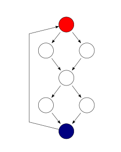
Another way to define the cyclomatic complexity of a program is to look at its control-flow graph, a directed graph containing the basic blocks of the program, with an edge between two basic blocks if control may pass from the first to the second.
Cyclomatic complexity may be applied to several such programs or subprograms at the same time (to all of the methods in a class, for example).
In these cases, P will equal the number of programs in question, and each subprogram will appear as a disconnected subset of the graph.
The set of all even subgraphs of a graph is closed under symmetric difference, and may thus be viewed as a vector space over GF(2).
which is read as "the rank of the first homology group of the graph G relative to the terminal nodes t".
This is a technical way of saying "the number of linearly independent paths through the flow graph from an entry to an exit", where: This cyclomatic complexity can be calculated.
It may also be computed via absolute Betti number by identifying the terminal nodes on a given component, or drawing paths connecting the exits to the entrance.
If a (connected) control-flow graph is considered a one-dimensional CW complex called
The fundamental group counts how many loops there are through the graph up to homotopy, aligning as expected.
In his presentation "Software Quality Metrics to Identify Risk"[8] for the Department of Homeland Security, Tom McCabe introduced the following categorization of cyclomatic complexity: One of McCabe's original applications was to limit the complexity of routines during program development.
[2] This practice was adopted by the NIST Structured Testing methodology, which observed that since McCabe's original publication, the figure of 10 had received substantial corroborating evidence.
However, it also noted that in some circumstances it may be appropriate to relax the restriction and permit modules with a complexity as high as 15.
[2] To calculate this measure, the original CFG is iteratively reduced by identifying subgraphs that have a single-entry and a single-exit point, which are then replaced by a single node.
This reduction corresponds to what a human would do if they extracted a subroutine from the larger piece of code.
[10] If a program is structured, then McCabe's reduction/condensation process reduces it to a single CFG node.
In contrast, if the program is not structured, the iterative process will identify the irreducible part.
It is useful because of two properties of the cyclomatic complexity, M, for a specific module: All three of the above numbers may be equal: branch coverage
Considering the example above, each time an additional if-then-else statement is added, the number of possible paths grows by a factor of 2.
As the program grows in this fashion, it quickly reaches the point where testing all of the paths becomes impractical.
In most cases, this number of tests is adequate to exercise all the relevant paths of the function.
Multiple studies have investigated the correlation between McCabe's cyclomatic complexity number with the frequency of defects occurring in a function or method.
However, the correlation between cyclomatic complexity and program size (typically measured in lines of code) has been demonstrated many times.
Les Hatton has claimed[13] that complexity has the same predictive ability as lines of code.
Studies that controlled for program size (i.e., comparing modules that have different complexities but similar size) are generally less conclusive, with many finding no significant correlation, while others do find correlation.
Some researchers question the validity of the methods used by the studies finding no correlation.
[15] Since program size is not a controllable feature of commercial software, the usefulness of McCabe's number has been questioned.
[11] The essence of this observation is that larger programs tend to be more complex and to have more defects.