Discrete wavelet transform

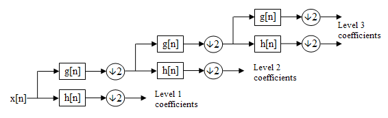
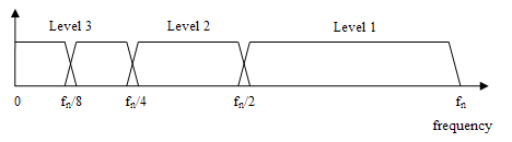
This decomposition is repeated to further increase the frequency resolution and the approximation coefficients decomposed with high- and low-pass filters and then down-sampled.

The locality of wavelets, coupled with the O(N) complexity, guarantees that the transform can be computed online (on a streaming basis).

This property is in sharp contrast to FFT, which requires access to the entire signal at once.

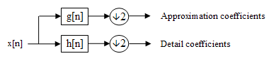
numbers, the Haar wavelet transform may be considered to pair up input values, storing the difference and passing the sum.

This process is repeated recursively, pairing up the sums to prove the next scale, which leads to

The most commonly used set of discrete wavelet transforms was formulated by the Belgian mathematician Ingrid Daubechies in 1988.

This formulation is based on the use of recurrence relations to generate progressively finer discrete samplings of an implicit mother wavelet function; each resolution is twice that of the previous scale.

Interest in this field has exploded since then, and many variations of Daubechies' original wavelets were developed.

WT) is a relatively recent enhancement to the discrete wavelet transform (DWT), with important additional properties: It is nearly shift invariant and directionally selective in two and higher dimensions.

WT is nonseparable but is based on a computationally efficient, separable filter bank (FB).

[5] Other forms of discrete wavelet transform include the Le Gall–Tabatabai (LGT) 5/3 wavelet developed by Didier Le Gall and Ali J. Tabatabai in 1988 (used in JPEG 2000 or JPEG XS ),[6][7][8] the Binomial QMF developed by Ali Naci Akansu in 1990,[9] the set partitioning in hierarchical trees (SPIHT) algorithm developed by Amir Said with William A. Pearlman in 1996,[10] the non- or undecimated wavelet transform (where downsampling is omitted), and the Newland transform (where an orthonormal basis of wavelets is formed from appropriately constructed top-hat filters in frequency space).

Complete Java code for a 1-D and 2-D DWT using Haar, Daubechies, Coiflet, and Legendre wavelets is available from the open source project: JWave.

Furthermore, a fast lifting implementation of the discrete biorthogonal CDF 9/7 wavelet transform in C, used in the JPEG 2000 image compression standard can be found here (archived 5 March 2012).

Due to the rate-change operators in the filter bank, the discrete WT is not time-invariant but actually very sensitive to the alignment of the signal in time.

[11] According to this algorithm, which is called a TI-DWT, only the scale parameter is sampled along the dyadic sequence 2^j (j∈Z) and the wavelet transform is calculated for each point in time.

[18] [19][20] It is shown that discrete wavelet transform (discrete in scale and shift, and continuous in time) is successfully implemented as analog filter bank in biomedical signal processing for design of low-power pacemakers and also in ultra-wideband (UWB) wireless communications.

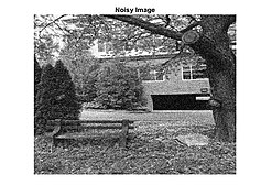
The following example provides three steps to remove unwanted white Gaussian noise from the noisy image shown.

Biorthogonal wavelets are commonly used in image processing to detect and filter white Gaussian noise,[22] due to their high contrast of neighboring pixel intensity values.

[24] Choosing other wavelets, levels, and thresholding strategies can result in different types of filtering.

Preliminary observations include: The DWT demonstrates the localization: the (1,1,1,1) term gives the average signal value, the (1,1,–1,–1) places the signal in the left side of the domain, and the (1,–1,0,0) places it at the left side of the left side, and truncating at any stage yields a downsampled version of the signal: The DFT, by contrast, expresses the sequence by the interference of waves of various frequencies – thus truncating the series yields a low-pass filtered version of the series: Notably, the middle approximation (2-term) differs.

From the frequency domain perspective, this is a better approximation, but from the time domain perspective it has drawbacks – it exhibits undershoot – one of the values is negative, though the original series is non-negative everywhere – and ringing, where the right side is non-zero, unlike in the wavelet transform.

This illustrates the kinds of trade-offs between these transforms, and how in some respects the DWT provides preferable behavior, particularly for the modeling of transients.

Prasanalakshmi B proposed a method [25] that uses the HL frequency sub-band in the middle-frequency coefficient sets LHx and HLx in a 5-level Discrete Wavelet Transform (DWT) transformed image.This algorithm chooses a coarser level of DWT in terms of imperceptibility and robustness to apply 4×4 block-based DCT on them.

The subcomponent LL1 is decomposed and critically subsampled to obtain the following coarser-scaled wavelet components.

Embedding the watermark in the middle-level frequency sub-bands LLx gives a high degree of imperceptibility and robustness.

Then, the block base DCT is performed on these selected DWT coefficient sets and embeds pseudorandom sequences in middle frequencies.

Decomposition is performed till 5-levels and the frequency subcomponents {HH1, HL1, LH1,{{HH2, HL2, LH2, {HH3, HL3, LH3, {HH4, HL4, LH4, {HH5, HL5, LH5, LL5}}}}}} are obtained by computing the fifth level DWT of the image I.

Two uncorrelated pseudorandom sequences are generated from the key obtained from the palm vein.

Embed the two pseudorandom sequences with a gain factor α in the DCT-transformed 4x4 blocks of the selected DWT coefficient sets of the host image.

Inverse DCT (IDCT) is done on each block after its mid-band coefficients have been modified to embed the watermark bits.