Fourier series
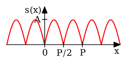
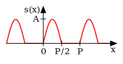
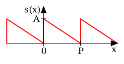
The figures below illustrate some partial Fourier series results for the components of a square wave.
Some of the more powerful and elegant approaches are based on mathematical ideas and tools that were not available in Fourier's time.
Many other Fourier-related transforms have since been defined, extending his initial idea to many applications and birthing an area of mathematics called Fourier analysis.
The Fourier series is named in honor of Jean-Baptiste Joseph Fourier (1768–1830), who made important contributions to the study of trigonometric series, after preliminary investigations by Leonhard Euler, Jean le Rond d'Alembert, and Daniel Bernoulli.
[A] Fourier introduced the series for the purpose of solving the heat equation in a metal plate, publishing his initial results in his 1807 Mémoire sur la propagation de la chaleur dans les corps solides (Treatise on the propagation of heat in solid bodies), and publishing his Théorie analytique de la chaleur (Analytical theory of heat) in 1822.
Through Fourier's research the fact was established that an arbitrary (at first, continuous[3] and later generalized to any piecewise-smooth[4]) function can be represented by a trigonometric series.
[5] Early ideas of decomposing a periodic function into the sum of simple oscillating functions date back to the 3rd century BC, when ancient astronomers proposed an empiric model of planetary motions, based on deferents and epicycles.
From a modern point of view, Fourier's results are somewhat informal, due to the lack of a precise notion of function and integral in the early nineteenth century.
Later, Peter Gustav Lejeune Dirichlet[7] and Bernhard Riemann[8][9][10] expressed Fourier's results with greater precision and formality.
Although the original motivation was to solve the heat equation, it later became obvious that the same techniques could be applied to a wide array of mathematical and physical problems, and especially those involving linear differential equations with constant coefficients, for which the eigensolutions are sinusoids.
This immediately gives any coefficient ak of the trigonometric series for φ(y) for any function which has such an expansion.
In what sense that is actually true is a somewhat subtle issue and the attempts over many years to clarify this idea have led to important discoveries in the theories of convergence, function spaces, and harmonic analysis.
When Fourier submitted a later competition essay in 1811, the committee (which included Lagrange, Laplace, Malus and Legendre, among others) concluded: ...the manner in which the author arrives at these equations is not exempt of difficulties and...his analysis to integrate them still leaves something to be desired on the score of generality and even rigour.
The example generalizes and one may compute ζ(2n), for any positive integer n. The Fourier series of a complex-valued P-periodic function
, a trigonometric series can also represent the intermediate frequencies and/or non-sinusoidal functions because of the infinite number of terms.
represents time, the coefficient sequence is called a frequency domain representation.
Square brackets are often used to emphasize that the domain of this function is a discrete set of frequencies.
Another commonly used frequency domain representation uses the Fourier series coefficients to modulate a Dirac comb: where
[C] Some common pairs of periodic functions and their Fourier series coefficients are shown in the table below.
This table shows some mathematical operations in the time domain and the corresponding effect in the Fourier series coefficients.
One of the interesting properties of the Fourier transform which we have mentioned, is that it carries convolutions to pointwise products.
to be the sphere with the usual metric, in which case the Fourier basis consists of spherical harmonics.
This generalization yields the usual Fourier transform when the underlying locally compact Abelian group is
For two-dimensional arrays with a staggered appearance, half of the Fourier series coefficients disappear, due to additional symmetry.
This kind of function can be, for example, the effective potential that one electron "feels" inside a periodic crystal.
in order to calculate the volume element in the original rectangular coordinate system.
(it may be advantageous for the sake of simplifying calculations, to work in such a rectangular coordinate system, in which it just so happens that
Because of the least squares property, and because of the completeness of the Fourier basis, we obtain an elementary convergence result.
The uniform boundedness principle yields a simple non-constructive proof of this fact.
In 1922, Andrey Kolmogorov published an article titled Une série de Fourier-Lebesgue divergente presque partout in which he gave an example of a Lebesgue-integrable function whose Fourier series diverges almost everywhere.


![{\displaystyle (-\pi ,\pi ]}](https://wikimedia.org/api/rest_v1/media/math/render/svg/7fbb1843079a9df3d3bbcce3249bb2599790de9c)