HSL and HSV
Note that while "hue" in HSL and HSV refers to the same attribute, their definitions of "saturation" differ dramatically.
Because HSL and HSV are simple transformations of device-dependent RGB models, the physical colors they define depend on the colors of the red, green, and blue primaries of the device or of the particular RGB space, and on the gamma correction used to represent the amounts of those primaries.
[1] Both of these representations are used widely in computer graphics, and one or the other of them is often more convenient than RGB, but both are also criticized for not adequately separating color-making attributes, or for their lack of perceptual uniformity.
Mixing these pure colors with black – producing so-called shades – leaves saturation unchanged.
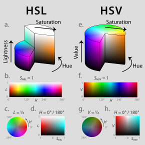
Because these definitions of saturation – in which very dark (in both models) or very light (in HSL) near-neutral colors are considered fully saturated (for instance, from the bottom right in the sliced HSL cylinder or from the top right) – conflict with the intuitive notion of color purity, often a conic or biconic solid is drawn instead (fig.
In the same issue, Joblove and Greenberg[11] described the HSL model – whose dimensions they labeled hue, relative chroma, and intensity – and compared it to HSV (fig.
[12][13][14][15] The dimensions of the HSL and HSV geometries – simple transformations of the not-perceptually-based RGB model – are not directly related to the photometric color-making attributes of the same names, as defined by scientists such as the CIE or ASTM.
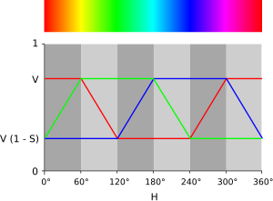
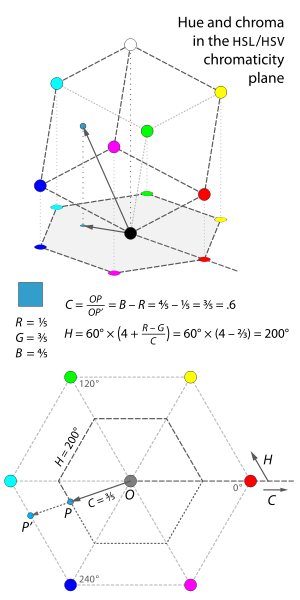
The HSL and HSV model-builders took an RGB cube – with constituent amounts of red, green, and blue light in a color denoted R, G, B ∈ [0, 1][E] – and tilted it on its corner, so that black rested at the origin with white directly above it along the vertical axis, then measured the hue of the colors in the cube by their angle around that axis, starting with red at 0°.
To make our definitions easier to write, we'll define these maximum, minimum, and chroma component values as M, m, and C, respectively.
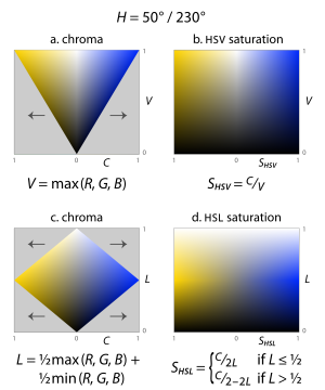
[11] To solve problems such as these, the HSL and HSV models scale the chroma so that it always fits into the range [0, 1] for every combination of hue and lightness or value, calling the new attribute saturation in both cases (fig.
Instead of presenting color choice or modification interfaces to end users, the goal of HSI is to facilitate separation of shapes in an image.
[28] Using the same name for these three different definitions of saturation leads to some confusion, as the three attributes describe substantially different color relationships; in HSV and HSI, the term roughly matches the psychometric definition, of a chroma of a color relative to its own lightness, but in HSL it does not come close.
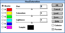
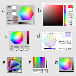
[K] The original purpose of HSL and HSV and similar models, and their most common current application, is in color selection tools.
The latter type of GUI exhibits great variety, because of the choice of cylinders, hexagonal prisms, or cones/bicones that the models suggest (see the diagram near the top of the page).
The CSS 3 specification allows web authors to specify colors for their pages directly with HSL coordinates.
For example, the popular GIS program ArcGIS historically applied customizable HSV-based gradients to numerical geographical data.
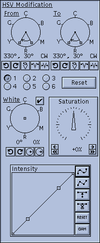
The image editor Picture Window Pro includes a "color correction" tool which affords complex remapping of points in a hue/saturation plane relative to either HSL or HSV space.
These have been copied widely, but several imitators use the HSL (e.g. PhotoImpact, Paint Shop Pro) or HSV geometries instead.
[28] Starting in the late 1970s, transformations like HSV or HSI were used as a compromise between effectiveness for segmentation and computational complexity.
They can be thought of as similar in approach and intent to the neural processing used by human color vision, without agreeing in particulars: if the goal is object detection, roughly separating hue, lightness, and chroma or saturation is effective, but there is no particular reason to strictly mimic human color response.
CIELAB L* is a CIE-defined achromatic lightness quantity (dependent solely on the perceptually achromatic luminance Y, but not the mixed-chromatic components X or Z, of the CIEXYZ colorspace from which the sRGB colorspace itself is derived), and it is plain that this appears similar in perceptual lightness to the original color image.
Though none of the dimensions in these spaces match their perceptual analogs, the value of HSV and the saturation of HSL are particular offenders.
Such perversities led Cynthia Brewer, expert in color scheme choices for maps and information displays, to tell the American Statistical Association: Computer science offers a few poorer cousins to these perceptual spaces that may also turn up in your software interface, such as HSV and HLS.
If much tweaking is required to achieve the desired effect, the system offers little benefit over grappling with raw specifications in RGB or CMY.
For instance, rotating the hue of a pure dark blue toward green will also reduce its perceived chroma, and increase its perceived lightness (the latter is grayer and lighter), but the same hue rotation will have the opposite impact on lightness and chroma of a lighter bluish-green – to (the latter is more colorful and slightly darker).
Notice how the hue-shifted middle version without such a correction dramatically changes the perceived lightness relationships between colors in the image.
[41] Charles Poynton, digital video expert, lists the above problems with HSL and HSV in his Color FAQ, and concludes that: HSB and HLS were developed to specify numerical Hue, Saturation and Brightness (or Hue, Lightness and Saturation) in an age when users had to specify colors numerically.
Finally, we can find R, G, and B by adding the same amount to each component, to match lightness: The polygonal piecewise functions can be somewhat simplified by clever use of minimum and maximum values as well as the remainder operation.
24 can help to get intuition about this): Given an HSI color with hue H ∈ [0°, 360°), saturation SI ∈ [0, 1], and intensity I ∈ [0, 1], we can use the same strategy, in a slightly different order: Where
Finally, we can find R, G, and B by adding the same amount to each component, to match lightness: Given a color with hue H ∈ [0°, 360°), chroma C ∈ [0, 1], and luma Y′601 ∈ [0, 1],[U] we can again use the same strategy.


- SGI IRIX 5, c. 1995 ;
- Adobe Photoshop , c. 1990 ;
- IBM OS/2 Warp 3, c. 1994 ;
- Apple Macintosh System 7 , c. 1996 ;
- Fractal Design Painter , c. 1993 ;
- Microsoft Windows 3.1 , c. 1992 ;
- NeXTSTEP , c. 1995 .