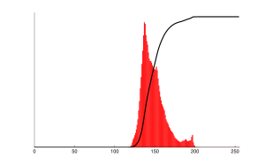
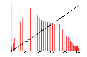
Histogram equalization
Histogram equalization accomplishes this by effectively spreading out the highly populated intensity values which are used to degrade image contrast.
The method is useful in images with backgrounds and foregrounds that are both bright or both dark.
In particular, the method can lead to better views of bone structure in x-ray images, and to better detail in photographs that are either over or under-exposed.
A key advantage of the method is that it is a fairly straightforward technique adaptive to the input image and an invertible operator.
It may increase the contrast of background noise, while decreasing the usable signal.
In scientific imaging where spatial correlation is more important than intensity of signal (such as separating DNA fragments of quantized length), the small signal-to-noise ratio usually hampers visual detections.
For example, if applied to 8-bit image displayed with 8-bit gray-scale palette it will further reduce color depth (number of unique shades of gray) of the image.
Histogram equalization will work the best when applied to images with much higher color depth than palette size, like continuous data or 16-bit gray-scale images.
In most cases palette change is better as it preserves the original data.
The goal of these methods, especially MBOBHE, is to improve the contrast without producing brightness mean-shift and detail loss artifacts by modifying the HE algorithm.
[1] A signal transform equivalent to histogram equalization also seems to happen in biological neural networks so as to maximize the output firing rate of the neuron as a function of the input statistics.
These methods seek to adjust the image to make it easier to analyze or improve visual quality (e.g., retinex) The back projection (or "project") of a histogrammed image is the re-application of the modified histogram to the original image, functioning as a look-up table for pixel brightness values.
For each group of pixels taken from the same position from all input single-channel images, the function puts the histogram bin value to the destination image, where the coordinates of the bin are determined by the values of pixels in this input group.
In terms of statistics, the value of each output image pixel characterizes the probability that the corresponding input pixel group belongs to the object whose histogram is used.
[3] Consider a discrete grayscale image {x} and let ni be the number of occurrences of gray level i.
being in fact the image's histogram for pixel value i, normalized to [0,1].
Let us also define the cumulative distribution function corresponding to i as which is also the image's accumulated normalized histogram.
Such an image would have a linearized cumulative distribution function (CDF) across the value range, i.e. for some constant
The properties of the CDF allow us to perform such a transform (see Inverse distribution function); it is defined as where
In order to map the values back into their original range, the following simple transformation needs to be applied on the result: A more detailed derivation is provided in University of California, Irvine Math 77C - Histogram Equalization.
An intuitive and popular method[4] is applying the round operation: However, detailed analysis results in slightly different formulation.
However it can also be used on color images by applying the same method separately to the Red, Green and Blue components of the RGB color values of the image.
However, applying the same method on the Red, Green, and Blue components of an RGB image may yield dramatic changes in the image's color balance since the relative distributions of the color channels change as a result of applying the algorithm.
Trahanias and Venetsanopoulos applied histogram equalization in 3D color space[6] However, it results in "whitening" where the probability of bright pixels are higher than that of dark ones.
[7] Han et al. proposed to use a new cdf defined by the iso-luminance plane, which results in uniform gray distribution.
Pixel values that have a zero count are excluded for the sake of brevity.
Again, pixel values that do not contribute to an increase in the cdf are excluded for brevity.
The cdf of 64 for value 154 coincides with the number of pixels in the image.
The general histogram equalization formula is: where cdfmin is the minimum non-zero value of the cumulative distribution function (in this case 1), M × N gives the image's number of pixels (for the example above 64, where M is width and N the height) and L is the number of grey levels used (in most cases, like this one, 256).
Note that to scale values in the original data that are above 0 to the range 1 to L-1, inclusive, the above equation would instead be: where cdf(v) > 0.