Interpolation
In the mathematical field of numerical analysis, interpolation is a type of estimation, a method of constructing (finding) new data points based on the range of a discrete set of known data points.
[1][2] In engineering and science, one often has a number of data points, obtained by sampling or experimentation, which represent the values of a function for a limited number of values of the independent variable.
Suppose the formula for some given function is known, but too complicated to evaluate efficiently.
The resulting gain in simplicity may outweigh the loss from interpolation error and give better performance in calculation process.
We describe some methods of interpolation, differing in such properties as: accuracy, cost, number of data points needed, and smoothness of the resulting interpolant function.
Generally, linear interpolation takes two data points, say (xa,ya) and (xb,yb), and the interpolant is given by: This previous equation states that the slope of the new line between
Denote the function which we want to interpolate by g, and suppose that x lies between xa and xb and that g is twice continuously differentiable.
Furthermore, polynomial interpolation may exhibit oscillatory artifacts, especially at the end points (see Runge's phenomenon).
However, these maxima and minima may exceed the theoretical range of the function; for example, a function that is always positive may have an interpolant with negative values, and whose inverse therefore contains false vertical asymptotes.
More generally, the shape of the resulting curve, especially for very high or low values of the independent variable, may be contrary to commonsense; that is, to what is known about the experimental system which has generated the data points.
These disadvantages can be reduced by using spline interpolation or restricting attention to Chebyshev polynomials.
The natural cubic spline interpolating the points in the table above is given by In this case we get f(2.5) = 0.5972.
This is completely mitigated by using splines of compact support, such as are implemented in Boost.Math and discussed in Kress.
[3] Depending on the underlying discretisation of fields, different interpolants may be required.
In contrast to other interpolation methods, which estimate functions on target points, mimetic interpolation evaluates the integral of fields on target lines, areas or volumes, depending on the type of field (scalar, vector, pseudo-vector or pseudo-scalar).
As a result, mimetic interpolation conserves line, area and volume integrals.
Given any interpolant that satisfies a set of constraints, TFC derives a functional that represents the entire family of interpolants satisfying those constraints, including those that are discontinuous or partially defined.
Consequently, TFC transforms constrained optimization problems into equivalent unconstrained formulations.
This transformation has proven highly effective in the solution of differential equations.
This simplifies solving various types of equations and significantly improves the efficiency and accuracy of methods like Physics-Informed Neural Networks (PINNs).
TFC offers advantages over traditional methods like Lagrange multipliers and spectral methods by directly addressing constraints analytically and avoiding iterative procedures, although it cannot currently handle inequality constraints.
In general, an interpolant need not be a good approximation, but there are well known and often reasonable conditions where it will.
(four times continuously differentiable) then cubic spline interpolation has an error bound given by
Many popular interpolation tools are actually equivalent to particular Gaussian processes.
In the geostatistics community Gaussian process regression is also known as Kriging.
This idea leads to the displacement interpolation problem used in transportation theory.
An early and fairly elementary discussion on this subject can be found in Rabiner and Crochiere's book Multirate Digital Signal Processing.
In curve fitting problems, the constraint that the interpolant has to go exactly through the data points is relaxed.
It is only required to approach the data points as closely as possible (within some other constraints).
mapping to a Banach space, then the problem is treated as "interpolation of operators".
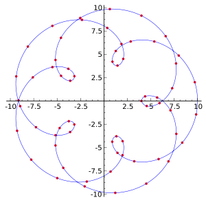


Black and red / yellow / green / blue dots correspond to the interpolated point and neighbouring samples, respectively.
Their heights above the ground correspond to their values.