k-nearest neighbors algorithm

In statistics, the k-nearest neighbors algorithm (k-NN) is a non-parametric supervised learning method.

In k-NN regression, also known as nearest neighbor smoothing, the output is the property value for the object.

Since this algorithm relies on distance, if the features represent different physical units or come in vastly different scales, then feature-wise normalizing of the training data can greatly improve its accuracy.

In the context of gene expression microarray data, for example, k-NN has been employed with correlation coefficients, such as Pearson and Spearman, as a metric.

[5] Often, the classification accuracy of k-NN can be improved significantly if the distance metric is learned with specialized algorithms such as Large Margin Nearest Neighbor or Neighbourhood components analysis.

A drawback of the basic "majority voting" classification occurs when the class distribution is skewed.

[6] One way to overcome this problem is to weight the classification, taking into account the distance from the test point to each of its k nearest neighbors.

For example, in a self-organizing map (SOM), each node is a representative (a center) of a cluster of similar points, regardless of their density in the original training data.

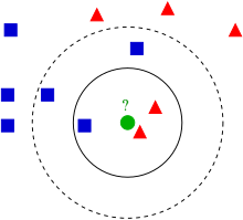
The best choice of k depends upon the data; generally, larger values of k reduces effect of the noise on the classification,[7] but make boundaries between classes less distinct.

A particularly popular[citation needed] approach is the use of evolutionary algorithms to optimize feature scaling.

[citation needed] In binary (two class) classification problems, it is helpful to choose k to be an odd number as this avoids tied votes.

An analogous result on the strong consistency of weighted nearest neighbour classifiers also holds.

With optimal weights the dominant term in the asymptotic expansion of the excess risk is

Using an approximate nearest neighbor search algorithm makes k-NN computationally tractable even for large data sets.

Many nearest neighbor search algorithms have been proposed over the years; these generally seek to reduce the number of distance evaluations actually performed.

[14] For multi-class k-NN classification, Cover and Hart (1967) prove an upper bound error rate of

denote the k nearest neighbour classifier based on a training set of size n. Under certain regularity conditions, the excess risk yields the following asymptotic expansion[11]

The K-nearest neighbor classification performance can often be significantly improved through (supervised) metric learning.

Popular algorithms are neighbourhood components analysis and large margin nearest neighbor.

When the input data to an algorithm is too large to be processed and it is suspected to be redundant (e.g. the same measurement in both feet and meters) then the input data will be transformed into a reduced representation set of features (also named features vector).

If the features extracted are carefully chosen it is expected that the features set will extract the relevant information from the input data in order to perform the desired task using this reduced representation instead of the full size input.

An example of a typical computer vision computation pipeline for face recognition using k-NN including feature extraction and dimension reduction pre-processing steps (usually implemented with OpenCV): For high-dimensional data (e.g., with number of dimensions more than 10) dimension reduction is usually performed prior to applying the k-NN algorithm in order to avoid the effects of the curse of dimensionality.

[18] For very-high-dimensional datasets (e.g. when performing a similarity search on live video streams, DNA data or high-dimensional time series) running a fast approximate k-NN search using locality sensitive hashing, "random projections",[19] "sketches"[20] or other high-dimensional similarity search techniques from the VLDB toolbox might be the only feasible option.

Nearest neighbor rules in effect implicitly compute the decision boundary.

White areas correspond to the unclassified regions, where 5NN voting is tied (for example, if there are two green, two red and one blue points among 5 nearest neighbors).

The crosses are the class-outliers selected by the (3,2)NN rule (all the three nearest neighbors of these instances belong to other classes); the squares are the prototypes, and the empty circles are the absorbed points.

The left bottom corner shows the numbers of the class-outliers, prototypes and absorbed points for all three classes.

5 shows that the 1NN classification map with the prototypes is very similar to that with the initial data set.

This algorithm works as follows: The distance to the kth nearest neighbor can also be seen as a local density estimate and thus is also a popular outlier score in anomaly detection.

The larger the distance to the k-NN, the lower the local density, the more likely the query point is an outlier.