Time series
Examples of time series are heights of ocean tides, counts of sunspots, and the daily closing value of the Dow Jones Industrial Average.
The parametric approaches assume that the underlying stationary stochastic process has a certain structure which can be described using a small number of parameters (for example, using an autoregressive or moving-average model).
Methods of time series analysis may also be divided into linear and non-linear, and univariate and multivariate.
In the context of statistics, econometrics, quantitative finance, seismology, meteorology, and geophysics the primary goal of time series analysis is forecasting.
Other applications are in data mining, pattern recognition and machine learning, where time series analysis can be used for clustering,[2][3][4] classification,[5] query by content,[6] anomaly detection as well as forecasting.
The total number of deaths declined in every year until the mid-1980s, after which there were occasional increases, often proportionately - but not absolutely - quite large.
[9] Visual tools that represent time series data as heat map matrices can help overcome these challenges.
This approach may be based on harmonic analysis and filtering of signals in the frequency domain using the Fourier transform, and spectral density estimation.
Its development was significantly accelerated during World War II by mathematician Norbert Wiener, electrical engineers Rudolf E. Kálmán, Dennis Gabor and others for filtering signals from noise and predicting signal values at a certain point in time.
A related topic is regression analysis,[21][22] which focuses more on questions of statistical inference such as how much uncertainty is present in a curve that is fit to data observed with random errors.
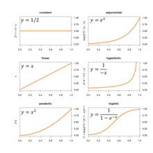
For processes that are expected to generally grow in magnitude one of the curves in the graphic (and many others) can be fitted by estimating their parameters.
Spline interpolation, however, yield a piecewise continuous function composed of many polynomials to model the data set.
Second, the target function, call it g, may be unknown; instead of an explicit formula, only a set of points (a time series) of the form (x, g(x)) is provided.
For example, if g is an operation on the real numbers, techniques of interpolation, extrapolation, regression analysis, and curve fitting can be used.
For example, the audio signal from a conference call can be partitioned into pieces corresponding to the times during which each person was speaking.
Models for time series data can have many forms and represent different stochastic processes.
An additional set of extensions of these models is available for use where the observed time-series is driven by some "forcing" time-series (which may not have a causal effect on the observed series): the distinction from the multivariate case is that the forcing series may be deterministic or under the experimenter's control.
These models represent autoregressive conditional heteroskedasticity (ARCH) and the collection comprises a wide variety of representation (GARCH, TARCH, EGARCH, FIGARCH, CGARCH, etc.).
Here changes in variability are related to, or predicted by, recent past values of the observed series.
HMM models are widely used in speech recognition, for translating a time series of spoken words into text.
There are two sets of conditions under which much of the theory is built: Ergodicity implies stationarity, but the converse is not necessarily the case.
Situations where the amplitudes of frequency components change with time can be dealt with in time-frequency analysis which makes use of a time–frequency representation of a time-series or signal.