Lissajous curve
The resulting family of curves was investigated by Nathaniel Bowditch in 1815, and later in more detail in 1857 by Jules Antoine Lissajous (for whom it has been named).
Finally, the value of δ determines the apparent "rotation" angle of the figure, viewed as if it were actually a three-dimensional curve.
Lissajous figures where a = 1, b = N (N is a natural number) and are Chebyshev polynomials of the first kind of degree N. This property is exploited to produce a set of points, called Padua points, at which a function may be sampled in order to compute either a bivariate interpolation or quadrature of the function over the domain [−1,1] × [−1,1].
Prior to modern electronic equipment, Lissajous curves could be generated mechanically by means of a harmonograph.
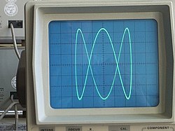
Two phase-shifted sinusoid inputs are applied to the oscilloscope in X-Y mode and the phase relationship between the signals is presented as a Lissajous figure.
The phase shifts are all negative so that delay semantics can be used with a causal LTI system (note that −270° is equivalent to +90°).
[citation needed] A Lissajous curve is used in experimental tests to determine if a device may be properly categorized as a memristor.
Examples include: Lissajous curves have been used in the past to graphically represent musical intervals through the use of the Harmonograph,[11] a device that consists of pendulums oscillating at different frequency ratios.
[12] Therefore, Lissajous curves have applications in music education by graphically representing differences between intervals and among tuning systems.


Middle: Input signal as a function of time.
Bottom: Resulting Lissajous curve when output is plotted as a function of the input.
In this particular example, because the output is 90 degrees out of phase from the input, the Lissajous curve is a circle, and is rotating counterclockwise.
