Marginal cost
On the short run, the firm has some costs that are fixed independently of the quantity of output (e.g. buildings, machinery).
The long run is defined as the length of time in which no input is fixed.
Everything, including building size and machinery, can be chosen optimally for the quantity of output that is desired.
Or, there may be increasing or decreasing returns to scale if technological or management productivity changes with the quantity.
In the short run, increasing production requires using more of the variable input — conventionally assumed to be labor.
[5] Denoting variable cost as VC, the constant wage rate as w, and labor usage as L, we have Here MPL is the ratio of increase in the quantity produced per unit increase in labour: i.e. ΔQ/ΔL, the marginal product of labor.
[7] Most recently, former Federal Reserve Vice-Chair Alan Blinder and colleagues conducted a survey of 200 executives of corporations with sales exceeding $10 million, in which they were asked, among other questions, about the structure of their marginal cost curves.
[8]: 106 Summing up the results, they wrote: ...many more companies state that they have falling, rather than rising, marginal cost curves.
While there are reasons to wonder whether respondents interpreted these questions about costs correctly, their answers paint an image of the cost structure of the typical firm that is very different from the one immortalized in textbooks.Many Post-Keynesian economists have pointed to these results as evidence in favor of their own heterodox theories of the firm, which generally assume that marginal cost is constant as production increases.
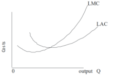
Economies of scale are said to exist if an additional unit of output can be produced for less than the average of all previous units – that is, if long-run marginal cost is below long-run average cost, so the latter is falling.
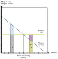
In perfectly competitive markets, firms decide the quantity to be produced based on marginal costs and sale price.
If the sale price is higher than the marginal cost, then they produce the unit and supply it.
So the production will be carried out until the marginal cost is equal to the sale price.
Since fixed costs do not vary with (depend on) changes in quantity, MC is ∆VC/∆Q.
Any such change would have no effect on the shape of the SRVC curve and therefore its slope MC at any point.
It is the marginal private cost that is used by business decision makers in their profit maximization behavior.
Externalities are costs (or benefits) that are not borne by the parties to the economic transaction.
In these cases, production or consumption of the good in question may differ from the optimum level.
In an equilibrium state, markets creating negative externalities of production will overproduce that good.
As a result, the socially optimal production level would be lower than that observed.
An example of such a public good, which creates a divergence in social and private costs, is the production of education.
In an equilibrium state, markets creating positive externalities of production will underproduce their good.
As a result, the socially optimal production level would be greater than that observed.
Therefore, (refer to "Average cost" labelled picture on the right side of the screen.
A firm can only produce so much but after the production of (n+1)th output reaches a minimum cost, the output produced after will only increase the average total cost (Nwokoye, Ebele & Ilechukwu, Nneamaka, 2018).
The firm is recommended to increase output to reach (Theory and Applications of Microeconomics, 2012).