Mixed model

[1][2] These models are useful in a wide variety of disciplines in the physical, biological and social sciences.

Further, they have their flexibility in dealing with missing values and uneven spacing of repeated measurements.

Often, ANOVA assumes the independence of observations within each group, however, this assumption may not hold in non-independent data, such as multilevel/hierarchical, longitudinal, or correlated datasets.

At the higher level, the school contains multiple individual students and teachers.

The school level influences the observations obtained from the students and teachers.

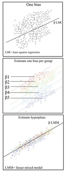
LMMs allow us to understand the important effects between and within levels while incorporating the corrections for standard errors for non-independence embedded in the data structure.

[4][5] In experimental fields such as social psychology, psycholinguistics, cognitive psychology (and neuroscience), where studies often involve multiple grouping variables, failing to account for random effects can lead to inflated Type I error rates and unreliable conclusions.

), ignoring variation in either of these grouping variables (e.g., by averaging over stimuli) can result in misleading conclusions.

In such cases, researchers can instead treat both participant and stimulus as random effects with LMMs, and in doing so, can correctly account for the variation in their data across multiple grouping variables.

Similarly, when analyzing data from comparative longitudinal surveys, failing to include random effects at all relevant levels—such as country and country-year—can significantly distort the results.

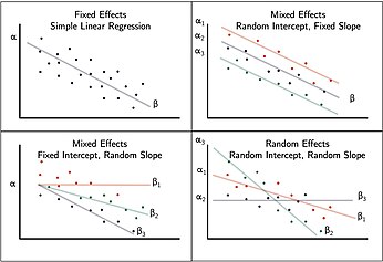
[8] Fixed effects encapsulate the tendencies/trends that are consistent at the levels of primary interest.

These effects are considered fixed because they are non-random and assumed to be constant for the population being studied.

While the hierarchy of the data set is typically obvious, the specific fixed effects that affect the average responses for all subjects must be specified.

Random effects introduce statistical variability at different levels of the data hierarchy.

[9][10][11] Ronald Fisher introduced random effects models to study the correlations of trait values between relatives.

Mixed models are applied in many disciplines where multiple correlated measurements are made on each unit of interest.

They are prominently used in research involving human and animal subjects in fields ranging from genetics to marketing, and have also been used in baseball [17] and industrial statistics.

LMM's have a constant-residual variance assumption that is sometimes violated when accounting for deeply associated continuous and binary traits.

The prior distribution for the category intercepts and slopes is described by the covariance matrix G. The joint density of

This is a consequence of the Gauss–Markov theorem when the conditional variance of the outcome is not scalable to the identity matrix.

One prominent recommendation in the context of confirmatory hypothesis testing[21] is to adopt a "maximal" random effects structure, including all possible random effects justified by the experimental design, as a means to control Type I error rates.

One method used to fit such mixed models is that of the expectation–maximization algorithm (EM) where the variance components are treated as unobserved nuisance parameters in the joint likelihood.

The solution to the mixed model equations is a maximum likelihood estimate when the distribution of the errors is normal.

[23][24] There are several other methods to fit mixed models, including using a mixed effect model (MEM) initially, and then Newton-Raphson (used by R package nlme[25]'s lme()), penalized least squares to get a profiled log likelihood only depending on the (low-dimensional) variance-covariance parameters of

Notably, while the canonical form proposed by Henderson is useful for theory, many popular software packages use a different formulation for numerical computation in order to take advantage of sparse matrix methods (e.g. lme4 and MixedModels.jl).

In the context of Bayesian methods, the brms package provides a user-friendly interface for fitting mixed models in R using Stan, allowing for the incorporation of prior distributions and the estimation of posterior distributions.

[27][28] In python, Bambi provides a similarly streamlined approach for fitting mixed effects models using PyMC.