Orthogonal trajectory

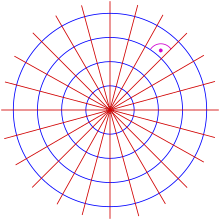
For example, the orthogonal trajectories of a pencil of concentric circles are the lines through their common center (see diagram).

Suitable methods for the determination of orthogonal trajectories are provided by solving differential equations.

The standard method establishes a first order ordinary differential equation and solves it by separation of variables.

Orthogonal trajectories are used in mathematics, for example as curved coordinate systems (i.e. elliptic coordinates) and appear in physics as electric fields and their equipotential curves.

Generally, one assumes that the pencil of curves is given implicitly by an equation where

yields Now it is assumed that equation (0) can be solved for parameter

One gets the differential equation of first order which is fulfilled by the given pencil of curves.

Because the slope of the orthogonal trajectory at a point

is the negative multiplicative inverse of the slope of the given curve at this point, the orthogonal trajectory satisfies the differential equation of first order This differential equation can (hopefully) be solved by a suitable method.

If the pencil of curves is represented implicitly in polar coordinates by one determines, alike the cartesian case, the parameter free differential equation of the pencil.

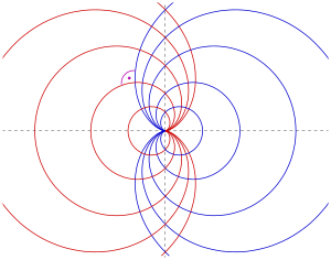
The differential equation of the orthogonal trajectories is then (see Redheffer & Port p. 65, Heuser, p. 120) Example: Cardioids: Elimination of

yields the differential equation of the given pencil: Hence the differential equation of the orthogonal trajectories is: After solving this differential equation by separation of variables one gets which describes the pencil of cardioids (red in diagram), symmetric to the given pencil.

For the determination of the isogonal trajectory one has to adjust the 3. step of the instruction above: The differential equation of the isogonal trajectory is: For the 1. example (concentric circles) and the angle

one gets This is a special kind of differential equation, which can be transformed by the substitution

into a differential equation, that can be solved by separation of variables.

After reversing the substitution one gets the equation of the solution: Introducing polar coordinates leads to the simple equation which describes logarithmic spirals (see diagram).

In case that the differential equation of the trajectories can not be solved by theoretical methods, one has to solve it numerically, for example by Runge–Kutta methods.