The Pareto distribution, named after the Italian civil engineer, economist, and sociologist Vilfredo Pareto,[2] is a power-law probability distribution that is used in description of social, quality control, scientific, geophysical, actuarial, and many other types of observable phenomena; the principle originally applied to describing the distribution of wealth in a society, fitting the trend that a large portion of wealth is held by a small fraction of the population.

Empirical observation has shown that this 80:20 distribution fits a wide range of cases, including natural phenomena[5] and human activities.

[6][7] If X is a random variable with a Pareto (Type I) distribution,[8] then the probability that X is greater than some number x, i.e., the survival function (also called tail function), is given by where xm is the (necessarily positive) minimum possible value of X, and α is a positive parameter.

From the definition, the cumulative distribution function of a Pareto random variable with parameters α and xm is It follows (by differentiation) that the probability density function is When plotted on linear axes, the distribution assumes the familiar J-shaped curve which approaches each of the orthogonal axes asymptotically.

All segments of the curve are self-similar (subject to appropriate scaling factors).

[9] The conditional probability distribution of a Pareto-distributed random variable, given the event that it is greater than or equal to a particular number

: In case of random variables that describe the lifetime of an object, this means that life expectancy is proportional to age, and is called the Lindy effect or Lindy's Law.

[citation needed] The geometric mean (G) is[11] The harmonic mean (H) is[11] The characteristic curved 'long tail' distribution, when plotted on a linear scale, masks the underlying simplicity of the function when plotted on a log-log graph, which then takes the form of a straight line with negative gradient: It follows from the formula for the probability density function that for x ≥ xm, Since α is positive, the gradient −(α + 1) is negative.

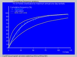
The Pareto distribution hierarchy is summarized in the next table comparing the survival functions (complementary CDF).

[15] In this section, the symbol xm, used before to indicate the minimum value of x, is replaced by σ.

Some special cases of Pareto Type (IV) are The finiteness of the mean, and the existence and the finiteness of the variance depend on the tail index α (inequality index γ).

If U is uniformly distributed on (0, 1), then applying inverse-transform method [19] is a bounded Pareto-distributed.

But if the distribution has symmetric structure with two slow decaying tails, Pareto could not do it.

The CDF of Zero Symmetric Pareto (ZSP) distribution is defined as following:

Hence, since x ≥ xm, we conclude that To find the estimator for α, we compute the corresponding partial derivative and determine where it is zero: Thus the maximum likelihood estimator for α is: The expected statistical error is:[22] Malik (1970)[23] gives the exact joint distribution of

Vilfredo Pareto originally used this distribution to describe the allocation of wealth among individuals since it seemed to show rather well the way that a larger portion of the wealth of any society is owned by a smaller percentage of the people in that society.

[4] This idea is sometimes expressed more simply as the Pareto principle or the "80-20 rule" which says that 20% of the population controls 80% of the wealth.

[24] As Michael Hudson points out (The Collapse of Antiquity [2023] p. 85 & n.7) "a mathematical corollary [is] that 10% would have 65% of the wealth, and 5% would have half the national wealth.” However, the 80-20 rule corresponds to a particular value of α, and in fact, Pareto's data on British income taxes in his Cours d'économie politique indicates that about 30% of the population had about 70% of the income.

[citation needed] The probability density function (PDF) graph at the beginning of this article shows that the "probability" or fraction of the population that owns a small amount of wealth per person is rather high, and then decreases steadily as wealth increases.

Both are a simple power law with a negative exponent, scaled so that their cumulative distributions equal 1.

This makes Zipf's probability density function derivable from Pareto's.

So a randomly selected person (or word, website link, or city) from a population (or language, internet, or country) has

Moreover, the following have been shown[34] to be mathematically equivalent: This does not apply only to income, but also to wealth, or to anything else that can be modeled by this distribution.

Price's square root law is sometimes offered as a property of or as similar to the Pareto distribution.

Note that in this case, the total and expected amount of wealth are not defined, and the rule only applies asymptotically to random samples.

The extended Pareto Principle mentioned above is a far more general rule.

Examples of the Lorenz curve for a number of Pareto distributions are shown in the graph on the right.

According to Oxfam (2016) the richest 62 people have as much wealth as the poorest half of the world's population.

[36] The Gini coefficient is a measure of the deviation of the Lorenz curve from the equidistribution line which is a line connecting [0, 0] and [1, 1], which is shown in black (α = ∞) in the Lorenz plot on the right.

Specifically, the Gini coefficient is twice the area between the Lorenz curve and the equidistribution line.