Probability distribution fitting
Probability distribution fitting or simply distribution fitting is the fitting of a probability distribution to a series of data concerning the repeated measurement of a variable phenomenon.
The aim of distribution fitting is to predict the probability or to forecast the frequency of occurrence of the magnitude of the phenomenon in a certain interval.
The distribution giving a close fit is supposed to lead to good predictions.
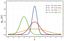
The selection of the appropriate distribution depends on the presence or absence of symmetry of the data set with respect to the central tendency.
The first two are very similar, while the last, with one degree of freedom, has "heavier tails" meaning that the values farther away from the mean occur relatively more often (i.e. the kurtosis is higher).
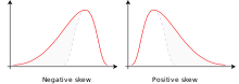
The following techniques of distribution fitting exist:[2] It is customary to transform data logarithmically to fit symmetrical distributions (like the normal and logistic) to data obeying a distribution that is positively skewed (i.e. skew to the right, with mean > mode, and with a right hand tail that is longer than the left hand tail), see lognormal distribution and the loglogistic distribution.
A similar effect can be achieved by taking the square root of the data.
To fit a symmetrical distribution to data obeying a negatively skewed distribution (i.e. skewed to the left, with mean < mode, and with a right hand tail this is shorter than the left hand tail) one could use the squared values of the data to accomplish the fit.
More generally one can raise the data to a power p in order to fit symmetrical distributions to data obeying a distribution of any skewness, whereby p < 1 when the skewness is positive and p > 1 when the skewness is negative.
The optimal value of p is to be found by a numerical method.
The numerical method may consist of assuming a range of p values, then applying the distribution fitting procedure repeatedly for all the assumed p values, and finally selecting the value of p for which the sum of squares of deviations of calculated probabilities from measured frequencies (chi squared) is minimum, as is done in CumFreq.
[6] The versatility of generalization makes it possible, for example, to fit approximately normally distributed data sets to a large number of different probability distributions,[7] while negatively skewed distributions can be fitted to square normal and mirrored Gumbel distributions.
[8] Skewed distributions can be inverted (or mirrored) by replacing in the mathematical expression of the cumulative distribution function (F) by its complement: F'=1-F, obtaining the complementary distribution function (also called survival function) that gives a mirror image.
Some probability distributions, like the exponential, do not support negative data values (X).
Yet, when negative data are present, such distributions can still be used replacing X by Y=X-Xm, where Xm is the minimum value of X.
This replacement represents a shift of the probability distribution in positive direction, i.e. to the right, because Xm is negative.
After completing the distribution fitting of Y, the corresponding X-values are found from X=Y+Xm, which represents a back-shift of the distribution in negative direction, i.e. to the left.
The technique of distribution shifting augments the chance to find a properly fitting probability distribution.
The option exists to use two different probability distributions, one for the lower data range, and one for the higher like for example the Laplace distribution.
The use of such composite (discontinuous) probability distributions can be opportune when the data of the phenomenon studied were obtained under two sets different conditions.
[6] Predictions of occurrence based on fitted probability distributions are subject to uncertainty, which arises from the following conditions: An estimate of the uncertainty in the first and second case can be obtained with the binomial probability distribution using for example the probability of exceedance Pe (i.e. the chance that the event X is larger than a reference value Xr of X) and the probability of non-exceedance Pn (i.e. the chance that the event X is smaller than or equal to the reference value Xr, this is also called cumulative probability).
This duality is the reason that the binomial distribution is applicable.
With the binomial distribution one can obtain a prediction interval.
The confidence or risk analysis may include the return period T=1/Pe as is done in hydrology.
This posterior can be used to update the probability mass function for a new sample
The variance of the newly obtained probability mass function can also be determined.
The variance for a Bayesian probability mass function can be defined as
This expression for the variance can be substantially simplified (assuming independently drawn samples).
The expression for variance involves an additional fit that includes the sample