Parks–McClellan filter design algorithm
[1] It was well known in both mathematics and engineering that the optimal response would exhibit an equiripple behavior and that the number of ripples could be counted using the Chebyshev approximation.
Several attempts to produce a design program for the optimal Chebyshev FIR filter were undertaken in the period between 1962 and 1971.
[1] This method obtained an equiripple frequency response with the maximum number of ripples by solving a set of nonlinear equations.
Another method introduced at the time implemented an optimal Chebyshev approximation, but the algorithm was limited to the design of relatively low-order filters.
[1] Similar to Herrmann's method, Ed Hofstetter presented an algorithm that designed FIR filters with as many ripples as possible.
At that time, DSP was an emerging field and as a result lectures often involved recently published research papers.
He brought the paper by Hofstetter, Oppenheim, and Siegel, back to Houston, thinking about the possibility of using the Chebyshev approximation theory to design FIR filters.
This ultimately led to the Parks–McClellan algorithm, which involved the theory of optimal Chebyshev approximation and an efficient implementation.
By the end of the spring semester, McClellan and Parks were attempting to write a variation of the Remez exchange algorithm for FIR filters.
The movement between bands was controlled by comparing the size of the errors at all the candidate extremal frequencies and taking the largest.
The following additional links provide information on the Parks–McClellan Algorithm, as well as on other research and papers written by James McClellan and Thomas Parks:
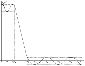
The y-axis is the frequency response H (ω) and the x-axis are the various radian frequencies, ω i . It can be noted that the two frequences marked on the x-axis, ω p and ω s . ω p indicates the pass band cutoff frequency and ω s indicates the stop band cutoff frequency. The ripple like plot on the upper left is the pass band ripple and the ripple on the bottom right is the stop band ripple. The two dashed lines on the top left of the graph indicate the δ p and the two dashed lines on the bottom right indicate the δ s . All other frequencies listed indicate the extremal frequencies of the frequency response plot. As a result, there are six extremal frequencies, and then we add the pass band and stop band frequencies to give a total of eight extremal frequencies on the plot.