Polar coordinate system
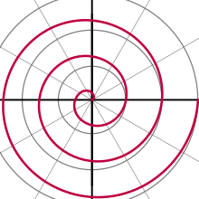
Polar coordinates are most appropriate in any context where the phenomenon being considered is inherently tied to direction and length from a center point in a plane, such as spirals.
The initial motivation for introducing the polar system was the study of circular and orbital motion.
From the 8th century AD onward, astronomers developed methods for approximating and calculating the direction to Mecca (qibla)—and its distance—from any location on the Earth.
[3] From the 9th century onward they were using spherical trigonometry and map projection methods to determine these quantities accurately.
The full history of the subject is described in Harvard professor Julian Lowell Coolidge's Origin of Polar Coordinates.
[5] Grégoire de Saint-Vincent and Bonaventura Cavalieri independently introduced the concepts in the mid-seventeenth century.
Cavalieri first used polar coordinates to solve a problem relating to the area within an Archimedean spiral.
Blaise Pascal subsequently used polar coordinates to calculate the length of parabolic arcs.
[6] In the journal Acta Eruditorum (1691), Jacob Bernoulli used a system with a point on a line, called the pole and polar axis respectively.
Bernoulli's work extended to finding the radius of curvature of curves expressed in these coordinates.
The actual term polar coordinates has been attributed to Gregorio Fontana and was used by 18th-century Italian writers.
The term appeared in English in George Peacock's 1816 translation of Lacroix's Differential and Integral Calculus.
[7][8] Alexis Clairaut was the first to think of polar coordinates in three dimensions, and Leonhard Euler was the first to actually develop them.
Angles in polar notation are generally expressed in either degrees or radians (2π rad being equal to 360°).
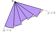
[9] The angle φ is defined to start at 0° from a reference direction, and to increase for rotations in either clockwise (cw) or counterclockwise (ccw) orientation.
The polar angles decrease towards negative values for rotations in the respectively opposite orientations.
Adding any number of full turns (360°) to the angular coordinate does not change the corresponding direction.
[12] Another convention, in reference to the usual codomain of the arctan function, is to allow for arbitrary nonzero real values of the radial component and restrict the polar angle to (−90°, 90°].
In polar form, the distance and angle coordinates are often referred to as the number's magnitude and argument respectively.
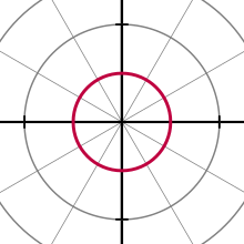
For the circle, line, and polar rose below, it is understood that there are no restrictions on the domain and range of the curve.
The variable a directly represents the length or amplitude of the petals of the rose, while k relates to their spatial frequency.
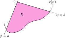
[17][18] The angular coordinate φ is expressed in radians throughout this section, which is the conventional choice when doing calculus.
Using Cartesian coordinates, an infinitesimal area element can be calculated as dA = dx dy.
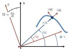
In planar particle dynamics these accelerations appear when setting up Newton's second law of motion in a rotating frame of reference.
For a particle in planar motion, one approach to attaching physical significance to these terms is based on the concept of an instantaneous co-rotating frame of reference.
An axis of rotation is set up that is perpendicular to the plane of motion of the particle, and passing through this origin.
They are most appropriate in any context where the phenomenon being considered is inherently tied to direction and length from a center point.
The initial motivation for the introduction of the polar system was the study of circular and orbital motion.
Polar coordinates are used often in navigation as the destination or direction of travel can be given as an angle and distance from the object being considered.
A prime example of this usage is the groundwater flow equation when applied to radially symmetric wells.