Primary production

Ecologists distinguish primary production as either net or gross, the former accounting for losses to processes such as cellular respiration, the latter not.

The following two equations are simplified representations of photosynthesis (top) and (one form of) chemosynthesis (bottom): In both cases, the end point is a polymer of reduced carbohydrate, (CH2O)n, typically molecules such as glucose or other sugars.

Primary production on land is a function of many factors, but principally local hydrology and temperature (the latter covaries to an extent with light, specifically photosynthetically active radiation (PAR), the source of energy for photosynthesis).

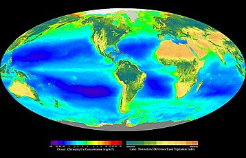
[citation needed] As shown in the animation, the boreal forests of Canada and Russia experience high productivity in June and July and then a slow decline through fall and winter.

Year-round, tropical forests in South America, Africa, Southeast Asia, and Indonesia have high productivity, not surprising with the abundant sunlight, warmth, and rainfall.

For example, the Amazon basin exhibits especially high productivity from roughly August through October - the period of the area's dry season.

[3] In a reversal of the pattern on land, in the oceans, almost all photosynthesis is performed by algae, with a small fraction contributed by vascular plants and other groups.

Unlike terrestrial ecosystems, the majority of primary production in the ocean is performed by free-living microscopic organisms called phytoplankton.

However, the availability of light, the source of energy for photosynthesis, and mineral nutrients, the building blocks for new growth, play crucial roles in regulating primary production in the ocean.

For practical purposes, the thickness of the photic zone is typically defined by the depth at which light reaches 1% of its surface value.

As long as there are adequate nutrients available, net primary production occurs whenever the mixed layer is shallower than the critical depth.

The most characteristic of these is the seasonal cycle (caused by the consequences of the Earth's axial tilt), although wind magnitudes additionally have strong spatial components.

In tropical regions, such as the gyres in the middle of the major basins, light may only vary slightly across the year, and mixing may only occur episodically, such as during large storms or hurricanes.

However, as long as the photic zone is deep enough, primary production may continue below the mixed layer where light-limited growth rates mean that nutrients are often more abundant.

Another factor relatively recently discovered to play a significant role in oceanic primary production is the micronutrient iron.

These areas are sometimes known as HNLC (High-Nutrient, Low-Chlorophyll) regions, because the scarcity of iron both limits phytoplankton growth and leaves a surplus of other nutrients.

Some scientists have suggested introducing iron to these areas as a means of increasing primary productivity and sequestering carbon dioxide from the atmosphere.

Field estimates rarely account for below ground productivity, herbivory, turnover, litterfall, volatile organic compounds, root exudates, and allocation to symbiotic microorganisms.

Gross primary production can be estimated from measurements of net ecosystem exchange (NEE) of carbon dioxide made by the eddy covariance technique.

Biomass increment based on stand specific allometry plus litterfall is considered a suitable although incomplete accounting of above-ground net primary production (ANPP).

The technique of using 14C incorporation (added as labelled Na2CO3) to infer primary production is most commonly used today because it is sensitive, and can be used in all ocean environments.

Gross primary production is best estimated using relatively short incubation times (1 hour or less), since the loss of incorporated 14C (by respiration and organic material excretion / exudation) will be more limited.

Loss processes can range between 10 and 60% of incorporated 14C according to the incubation period, ambient environmental conditions (especially temperature) and the experimental species used.

The methods based on stable isotopes and O2/Ar ratios have the advantage of providing estimates of respiration rates in the light without the need of incubations in the dark.

However, quantifying primary production at this scale is difficult because of the range of habitats on Earth, and because of the impact of weather events (availability of sunlight, water) on its variability.

Scaling ecosystem-level GPP estimations based on eddy covariance measurements of net ecosystem exchange (see above) to regional and global values using spatial details of different predictor variables, such as climate variables and remotely sensed fAPAR or LAI led to a terrestrial gross primary production of 123±8 Gt carbon (NOT carbon dioxide) per year during 1998-2005 [23] In areal terms, it was estimated that land production was approximately 426 g C m−2 yr−1 (excluding areas with permanent ice cover), while that for the oceans was 140 g C m−2 yr−1.

Present day primary productivity can be estimated through a variety of methodologies including ship-board measurements, satellites and terrestrial observatories.

One example is using barium, where barite concentrations in marine sediments rise in line with carbon export production at the surface.

The extensive degree of human use of the Planet's resources, mostly via land use, results in various levels of impact on actual NPP (NPPact).

Although in some regions, such as the Nile valley, irrigation has resulted in a considerable increase in primary production, in most of the Planet, there is a notable trend of NPP reduction due to land changes (ΔNPPLC) of 9.6% across global land-mass.