Self-organizing map
A self-organizing map (SOM) or self-organizing feature map (SOFM) is an unsupervised machine learning technique used to produce a low-dimensional (typically two-dimensional) representation of a higher-dimensional data set while preserving the topological structure of the data.
An SOM is a type of artificial neural network but is trained using competitive learning rather than the error-correction learning (e.g., backpropagation with gradient descent) used by other artificial neural networks.
[4] SOMs create internal representations reminiscent of the cortical homunculus[citation needed], a distorted representation of the human body, based on a neurological "map" of the areas and proportions of the human brain dedicated to processing sensory functions, for different parts of the body.
A map space consists of components called "nodes" or "neurons", which are arranged as a hexagonal or rectangular grid with two dimensions.
[5] The number of nodes and their arrangement are specified beforehand based on the larger goals of the analysis and exploration of the data.
While nodes in the map space stay fixed, training consists in moving weight vectors toward the input data (reducing a distance metric such as Euclidean distance) without spoiling the topology induced from the map space.
After training, the map can be used to classify additional observations for the input space by finding the node with the closest weight vector (smallest distance metric) to the input space vector.
The goal of learning in the self-organizing map is to cause different parts of the network to respond similarly to certain input patterns.
[6] The weights of the neurons are initialized either to small random values or sampled evenly from the subspace spanned by the two largest principal component eigenvectors.
When a training example is fed to the network, its Euclidean distance to all weight vectors is computed.
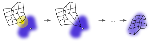
The neuron whose weight vector is most similar to the input is called the best matching unit (BMU).
The weights of the BMU and neurons close to it in the SOM grid are adjusted towards the input vector.
The update formula for a neuron v with weight vector Wv(s) is where s is the step index, t is an index into the training sample, u is the index of the BMU for the input vector D(t), α(s) is a monotonically decreasing learning coefficient; θ(u, v, s) is the neighborhood function which gives the distance between the neuron u and the neuron v in step s.[8] Depending on the implementations, t can scan the training data set systematically (t is 0, 1, 2...T-1, then repeat, T being the training sample's size), be randomly drawn from the data set (bootstrap sampling), or implement some other sampling method (such as jackknifing).
[6] At the beginning when the neighborhood is broad, the self-organizing takes place on the global scale.
When the neighborhood has shrunk to just a couple of neurons, the weights are converging to local estimates.
In some implementations, the learning coefficient α and the neighborhood function θ decrease steadily with increasing s, in others (in particular those where t scans the training data set) they decrease in step-wise fashion, once every T steps.
This process is repeated for each input vector for a (usually large) number of cycles λ.
The network winds up associating output nodes with groups or patterns in the input data set.
While representing input data as vectors has been emphasized in this article, any kind of object which can be represented digitally, which has an appropriate distance measure associated with it, and in which the necessary operations for training are possible can be used to construct a self-organizing map.
This includes matrices, continuous functions or even other self-organizing maps.
The variable names mean the following, with vectors in bold, The key design choices are the shape of the SOM, the neighbourhood function, and the learning rate schedule.
Notice in particular, that the update rate does not depend on where the point is in the Euclidean space, only on where it is in the SOM itself.
are close on the SOM, so they will always update in similar ways, even when they are far apart on the Euclidean space.
end up overlapping each other (such as if the SOM looks like a folded towel), they still do not update in similar ways.
Because in the training phase weights of the whole neighborhood are moved in the same direction, similar items tend to excite adjacent neurons.
This may be visualized by a U-Matrix (Euclidean distance between weight vectors of neighboring cells) of the SOM.
SOM may be considered a nonlinear generalization of Principal components analysis (PCA).
[17] It has been shown, using both artificial and real geophysical data, that SOM has many advantages[18][19] over the conventional feature extraction methods such as Empirical Orthogonal Functions (EOF) or PCA.
Nevertheless, there have been several attempts to modify the definition of SOM and to formulate an optimisation problem which gives similar results.