Differential geometry of surfaces

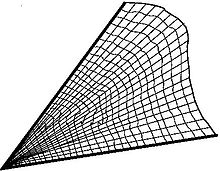
Surfaces naturally arise as graphs of functions of a pair of variables, and sometimes appear in parametric form or as loci associated to space curves.

These Lie groups can be used to describe surfaces of constant Gaussian curvature; they also provide an essential ingredient in the modern approach to intrinsic differential geometry through connections.

Monge laid down the foundations of their theory in his classical memoir L'application de l'analyse à la géometrie which appeared in 1795.

The nineteenth century was the golden age for the theory of surfaces, from both the topological and the differential-geometric point of view, with most leading geometers devoting themselves to their study.

Although conventions vary in their precise definition, these form a general class of subsets of three-dimensional Euclidean space (ℝ3) which capture part of the familiar notion of "surface."

[6][7][8] A regular surface in Euclidean space ℝ3 is a subset S of ℝ3 such that every point of S admits any of the following three concepts: local parametrizations, Monge patches, or implicit functions.

It is also useful to note an "intrinsic" definition of tangent vectors, which is typical of the generalization of regular surface theory to the setting of smooth manifolds.

The Christoffel symbols assign, to each local parametrization f : V → S, eight functions on V, defined by[22] They can also be defined by the following formulas, in which n is a unit normal vector field along f(V) and L, M, N are the corresponding components of the second fundamental form: The key to this definition is that ⁠∂f/∂u⁠, ⁠∂f/∂v⁠, and n form a basis of ℝ3 at each point, relative to which each of the three equations uniquely specifies the Christoffel symbols as coordinates of the second partial derivatives of f. The choice of unit normal has no effect on the Christoffel symbols, since if n is exchanged for its negation, then the components of the second fundamental form are also negated, and so the signs of Ln, Mn, Nn are left unchanged.

The Gauss equation is particularly noteworthy, as it shows that the Gaussian curvature can be computed directly from the first fundamental form, without the need for any other information; equivalently, this says that LN − M2 can actually be written as a function of E, F, G, even though the individual components L, M, N cannot.

[...] To our knowledge there is no simple geometric proof of the theorema egregium today.The Gauss-Codazzi equations can also be succinctly expressed and derived in the language of connection forms due to Élie Cartan.

For instance, the right-hand side can be recognized as the second coordinate of relative to the basis ⁠∂f/∂u⁠, ⁠∂f/∂v⁠, as can be directly verified using the definition of covariant differentiation by Christoffel symbols.

Curves on a surface which minimize length between the endpoints are called geodesics; they are the shape that an elastic band stretched between the two points would take.

A convenient way to understand the curvature comes from an ordinary differential equation, first considered by Gauss and later generalized by Jacobi, arising from the change of normal coordinates about two different points.

Gauss generalised these results to an arbitrary surface by showing that the integral of the Gaussian curvature over the interior of a geodesic triangle is also equal to this angle difference or excess.

This invariant is easy to compute combinatorially in terms of the number of vertices, edges, and faces of the triangles in the decomposition, also called a triangulation.

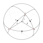
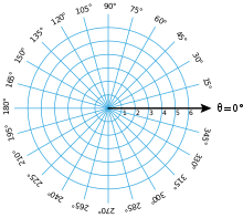
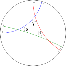
Gauss proved that, if Δ is a geodesic triangle on a surface with angles α, β and γ at vertices A, B and C, then In fact taking geodesic polar coordinates with origin A and AB, AC the radii at polar angles 0 and α: where the second equality follows from the Gauss–Jacobi equation and the fourth from Gauss's derivative formula in the orthogonal coordinates (r,θ).

Thus a closed Riemannian 2-manifold of non-positive curvature can never be embedded isometrically in E3; however, as Adriano Garsia showed using the Beltrami equation for quasiconformal mappings, this is always possible for some conformally equivalent metric.

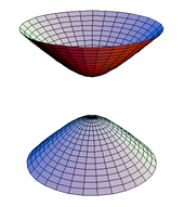
In other words, by multiplying the metric by a positive scaling factor, the Gaussian curvature can be made to take exactly one of these values (the sign of the Euler characteristic of M).

[77] Geodesics are straight lines and the geometry is encoded in the elementary formulas of trigonometry, such as the cosine rule for a triangle with sides a, b, c and angles α, β, γ: Flat tori can be obtained by taking the quotient of R2 by a lattice, i.e. a free Abelian subgroup of rank 2.

It is defined by points A, B, C on the sphere with sides BC, CA, AB formed from great circle arcs of length less than π.

[80] With respect to the coordinates (u, v) in the complex plane, the spherical metric becomes[81] The unit sphere is the unique closed orientable surface with constant curvature +1.

Non-Euclidean geometry[82] was first discussed in letters of Gauss, who made extensive computations at the turn of the nineteenth century which, although privately circulated, he decided not to put into print.

Because of their application in complex analysis and geometry, however, the models of Poincaré are the most widely used: they are interchangeable thanks to the Möbius transformations between the disk and the upper half-plane.

[d] The classical approach of Gauss to the differential geometry of surfaces was the standard elementary approach[89] which predated the emergence of the concepts of Riemannian manifold initiated by Bernhard Riemann in the mid-nineteenth century and of connection developed by Tullio Levi-Civita, Élie Cartan and Hermann Weyl in the early twentieth century.

The notion of connection, covariant derivative and parallel transport gave a more conceptual and uniform way of understanding curvature, which not only allowed generalisations to higher dimensional manifolds but also provided an important tool for defining new geometric invariants, called characteristic classes.

In the case of an embedded surface, the lift to an operator on vector fields, called the covariant derivative, is very simply described in terms of orthogonal projection.

As Ricci and Levi-Civita realised at the turn of the twentieth century, this process depends only on the metric and can be locally expressed in terms of the Christoffel symbols.

Equivalently curvature can be calculated directly at an infinitesimal level in terms of Lie brackets of lifted vector fields.

This enabled the curvature properties of the surface to be encoded in differential forms on the frame bundle and formulas involving their exterior derivatives.

Accounts of the classical theory are given in Eisenhart (2004), Kreyszig (1991) and Struik (1988); the more modern copiously illustrated undergraduate textbooks by Gray, Abbena & Salamon (2006), Pressley (2001) and Wilson (2008) might be found more accessible.