Sobel operator

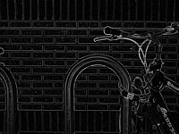
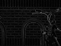
The Sobel operator, sometimes called the Sobel–Feldman operator or Sobel filter, is used in image processing and computer vision, particularly within edge detection algorithms where it creates an image emphasising edges.

It is named after Irwin Sobel and Gary M. Feldman, colleagues at the Stanford Artificial Intelligence Laboratory (SAIL).

Sobel and Feldman presented the idea of an "Isotropic 3 × 3 Image Gradient Operator" at a talk at SAIL in 1968.

[1] Technically, it is a discrete differentiation operator, computing an approximation of the gradient of the image intensity function.

The Sobel–Feldman operator is based on convolving the image with a small, separable, and integer-valued filter in the horizontal and vertical directions and is therefore relatively inexpensive in terms of computations.

On the other hand, the gradient approximation that it produces is relatively crude, in particular for high-frequency variations in the image.

The operator uses two 3×3 kernels which are convolved with the original image to calculate approximations of the derivatives – one for horizontal changes, and one for vertical.

In his text describing the origin of the operator,[1] Sobel shows different signs for these kernels.

However, approximations of these derivative functions can be defined at lesser or larger degrees of accuracy.

The Sobel–Feldman operator represents a rather inaccurate approximation of the image gradient, but is still of sufficient quality to be of practical use in many applications.

Thus as an example the 3D Sobel–Feldman kernel in z-direction: As a consequence of its definition, the Sobel operator can be implemented by simple means in both hardware and software: only eight image points around a point are needed to compute the corresponding result and only integer arithmetic is needed to compute the gradient vector approximation.

Applying convolution K to pixel group P can be represented in pseudocode as: where

It can be processed and viewed as though it is itself an image, with the areas of high gradient (the likely edges) visible as white lines.

The images below illustrate the change in the direction of the gradient on a grayscale circle.

The vertical edges on the left and right sides of the circle have an angle of 0 because there is no local change in

The horizontal edges at the top and bottom sides of the circle have angles of −⁠π/2⁠ and ⁠π/2⁠ respectively because there is no local change in

The negative angle for top edge signifies the transition is from a bright to dark region, and the positive angle for the bottom edge signifies a transition from a dark to bright region.

All other pixels are marked as black due to no local change in either

pixels with small rates of change can still have a large angle response.

As a result noise can have a large angle response which is typically undesired.

[3][4] Optimized 3D filter kernels up to a size of 5 x 5 x 5 have been presented there, but the most frequently used, with an error of about 0.2° is: This factors similarly: Scharr operators result from an optimization minimizing weighted mean squared angular error in the Fourier domain.

This optimization is done under the condition that resulting filters are numerically consistent.

The optimal 8 bit integer valued 3x3 filter stemming from Scharr's theory is A similar optimization strategy and resulting filters were also presented by Farid and Simoncelli.

In contrast to the work of Scharr, these filters are not enforced to be numerically consistent.

[7] Derivative filters based on arbitrary cubic splines were presented by Hast.

Larger schemes with even higher accuracy and optimized filter families for extended optical flow estimation have been presented in subsequent work by Scharr.

[10] Second order derivative filter sets have been investigated for transparent motion estimation.

[11] It has been observed that the larger the resulting kernels are, the better they approximate derivative-of-Gaussian filters.