Taxicab geometry
The name refers to the island of Manhattan, or generically any planned city with a rectangular grid of streets, in which a taxicab can only travel along grid directions.
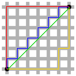
In taxicab geometry, the distance between any two points equals the length of their shortest grid path.
[1] This geometry has been used in regression analysis since the 18th century, and is often referred to as LASSO.
Its geometric interpretation dates to non-Euclidean geometry of the 19th century and is due to Hermann Minkowski.
The L1 metric was used in regression analysis, as a measure of goodness of fit, in 1757 by Roger Joseph Boscovich.
[2] The interpretation of it as a distance between points in a geometric space dates to the late 19th century and the development of non-Euclidean geometries.
Notably it appeared in 1910 in the works of both Frigyes Riesz and Hermann Minkowski.
The formalization of Lp spaces, which include taxicab geometry as a special case, is credited to Riesz.
[3] In developing the geometry of numbers, Hermann Minkowski established his Minkowski inequality, stating that these spaces define normed vector spaces.
[5] Thought of as an additional structure layered on Euclidean space, taxicab distance depends on the orientation of the coordinate system and is changed by Euclidean rotation of the space, but is unaffected by translation or axis-aligned reflections.
Taxicab geometry satisfies all of Hilbert's axioms (a formalization of Euclidean geometry) except that the congruence of angles cannot be defined to precisely match the Euclidean concept, and under plausible definitions of congruent taxicab angles, the side-angle-side axiom is not satisfied as in general triangles with two taxicab-congruent sides and a taxicab-congruent angle between them are not congruent triangles.
Whereas a Euclidean sphere is round and rotationally symmetric, under the taxicab distance, the shape of a sphere is a cross-polytope, the n-dimensional generalization of a regular octahedron, whose points
In two dimensional taxicab geometry, the sphere (called a circle) is a square oriented diagonally to the coordinate axes.
The image to the right shows in red the set of all points on a square grid with a fixed distance from the blue center.
As the grid is made finer, the red points become more numerous, and in the limit tend to a continuous tilted square.
Thus, in taxicab geometry, the value of the analog of the circle constant π, the ratio of circumference to diameter, is equal to 4.
A closed ball (or closed disk in the 2-dimensional case) is a filled-in sphere, the set of points at distance less than or equal to the radius from a specific center.
For cellular automata on a square grid, a taxicab disk is the von Neumann neighborhood of range r of its center.
A circle of radius r for the Chebyshev distance (L∞ metric) on a plane is also a square with side length 2r parallel to the coordinate axes, so planar Chebyshev distance can be viewed as equivalent by rotation and scaling to planar taxicab distance.
Whenever each pair in a collection of these circles has a nonempty intersection, there exists an intersection point for the whole collection; therefore, the Manhattan distance forms an injective metric space.
There are several theorems that guarantee triangle congruence in Euclidean geometry, namely Angle-Angle-Side (AAS), Angle-Side-Angle (ASA), Side-Angle-Side (SAS), and Side-Side-Side (SSS).
In taxicab geometry, however, only SASAS guarantees triangle congruence.
[11] Take, for example, two right isosceles taxicab triangles whose angles measure 45-90-45.
The two legs of both triangles have a taxicab length 2, but the hypotenuses are not congruent.
Having three congruent angles and two sides does not guarantee triangle congruence in taxicab geometry.
[12] This result is mainly due to the fact that the length of a line segment depends on its orientation in taxicab geometry.
[13] This approach appears in the signal recovery framework called compressed sensing.
Taxicab geometry can be used to assess the differences in discrete frequency distributions.
For example, in RNA splicing positional distributions of hexamers, which plot the probability of each hexamer appearing at each given nucleotide near a splice site, can be compared with L1-distance.
This is equivalent to measuring the area between the two distribution curves because the area of each segment is the absolute difference between the two curves' likelihoods at that point.