Aliasing
Aliasing is generally avoided by applying low-pass filters or anti-aliasing filters (AAF) to the input signal before sampling and when converting a signal from a higher to a lower sampling rate.
When a digital image is viewed, a reconstruction is performed by a display or printer device, and by the eyes and the brain.
An example of spatial aliasing is the moiré pattern observed in a poorly pixelized image of a brick wall.
[1] Temporal aliasing is a major concern in the sampling of video and audio signals.
To prevent this, an anti-aliasing filter is used to remove components above the Nyquist frequency prior to sampling.
In video or cinematography, temporal aliasing results from the limited frame rate, and causes the wagon-wheel effect, whereby a spoked wheel appears to rotate too slowly or even backwards.
Some of the most dramatic and subtle examples of aliasing occur when the signal being sampled also has periodic content.
Actual signals have a finite duration and their frequency content, as defined by the Fourier transform, has no upper bound.
Some amount of aliasing always occurs when such continuous functions over time are sampled.
Functions whose frequency content is bounded (bandlimited) have an infinite duration in the time domain.
Sinusoids are an important type of periodic function, because realistic signals are often modeled as the summation of many sinusoids of different frequencies and different amplitudes (for example, with a Fourier series or transform).
For example, a snapshot of the lower right frame of Fig.2 shows a component at the actual frequency
Aliasing matters when one attempts to reconstruct the original waveform from its samples.
The lower left frame of Fig.2 depicts the typical reconstruction result of the available samples.
exceeds the Nyquist frequency, the reconstruction matches the actual waveform (upper left frame).
The figures below offer additional depictions of aliasing, due to sampling.
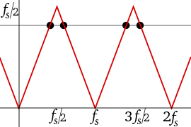
No matter what function we choose to change the amplitude vs frequency, the graph will exhibit symmetry between 0 and fs.
Folding is often observed in practice when viewing the frequency spectrum of real-valued samples, such as Fig.4.
That is typically approximated by filtering the original signal to attenuate high frequency components before it is sampled.
These attenuated high frequency components still generate low-frequency aliases, but typically at low enough amplitudes that they do not cause problems.
The filtered signal can subsequently be reconstructed, by interpolation algorithms, without significant additional distortion.
But the fidelity of a theoretical reconstruction (via the Whittaker–Shannon interpolation formula) is a customary measure of the effectiveness of sampling.
Historically the term aliasing evolved from radio engineering because of the action of superheterodyne receivers.
The first written use of the terms "alias" and "aliasing" in signal processing appears to be in a 1949 unpublished Bell Laboratories technical memorandum[4] by John Tukey and Richard Hamming.
The first published use of the term "aliasing" in this context is due to Blackman and Tukey in 1958.
[5] In their preface to the Dover reprint[6] of this paper, they point out that the idea of aliasing had been illustrated graphically by Stumpf[7] ten years prior.
The 1949 Bell technical report refers to aliasing as though it is a well-known concept, but does not offer a source for the term.
Aliasing occurs whenever the use of discrete elements to capture or produce a continuous signal causes frequency ambiguity.
The lack of parallax on viewer movement in 2D images and in 3-D film produced by stereoscopic glasses (in 3D films the effect is called "yawing", as the image appears to rotate on its axis) can similarly be seen as loss of angular resolution, all angular frequencies being aliased to 0 (constant).
A form of spatial aliasing can also occur in antenna arrays or microphone arrays used to estimate the direction of arrival of a wave signal, as in geophysical exploration by seismic waves.