Travelling salesman problem

Thus, it is possible that the worst-case running time for any algorithm for the TSP increases superpolynomially (but no more than exponentially) with the number of cities.

A handbook for travelling salesmen from 1832 mentions the problem and includes example tours through Germany and Switzerland, but contains no mathematical treatment.

[4] The general form of the TSP appears to have been first studied by mathematicians during the 1930s in Vienna and at Harvard, notably by Karl Menger, who defines the problem, considers the obvious brute-force algorithm, and observes the non-optimality of the nearest neighbour heuristic:

[6] Notable contributions were made by George Dantzig, Delbert Ray Fulkerson, and Selmer M. Johnson from the RAND Corporation, who expressed the problem as an integer linear program and developed the cutting plane method for its solution.

Halton, and John Hammersley published an article entitled "The Shortest Path Through Many Points" in the journal of the Cambridge Philosophical Society.

Great progress was made in the late 1970s and 1980, when Grötschel, Padberg, Rinaldi and others managed to exactly solve instances with up to 2,392 cities, using cutting planes and branch-and-bound.

Gerhard Reinelt published the TSPLIB in 1991, a collection of benchmark instances of varying difficulty, which has been used by many research groups for comparing results.

If no path exists between two cities, then adding a sufficiently long edge will complete the graph without affecting the optimal tour.

Traffic congestion, one-way streets, and airfares for cities with different departure and arrival fees are real-world considerations that could yield a TSP problem in asymmetric form.

[23] The traditional lines of attack for the NP-hard problems are the following: The most direct solution would be to try all permutations (ordered combinations) and see which one is cheapest (using brute-force search).

[26] Other approaches include: An exact solution for 15,112 German towns from TSPLIB was found in 2001 using the cutting-plane method proposed by George Dantzig, Ray Fulkerson, and Selmer M. Johnson in 1954, based on linear programming.

In April 2006 an instance with 85,900 points was solved using Concorde TSP Solver, taking over 136 CPU-years; see Applegate et al. (2006).

[35] The algorithm of Christofides and Serdyukov follows a similar outline but combines the minimum spanning tree with a solution of another problem, minimum-weight perfect matching.

[10] This algorithm looks at things differently by using a result from graph theory which helps improve on the lower bound of the TSP which originated from doubling the cost of the minimum spanning tree.

If we start with an initial solution made with a greedy algorithm, then the average number of moves greatly decreases again and is ⁠

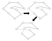
It involves the following steps: The most popular of the k-opt methods are 3-opt, as introduced by Shen Lin of Bell Labs in 1965.

In practice, it is often possible to achieve substantial improvement over 2-opt without the combinatorial cost of the general 3-opt by restricting the 3-changes to this special subset where two of the removed edges are adjacent.

Shen Lin and Brian Kernighan first published their method in 1972, and it was the most reliable heuristic for solving travelling salesman problems for nearly two decades.

More advanced variable-opt methods were developed at Bell Labs in the late 1980s by David Johnson and his research team.

ACS sends out a large number of virtual ant agents to explore many possible routes on the map.

The last two metrics appear, for example, in routing a machine that drills a given set of holes in a printed circuit board.

The Manhattan metric corresponds to a machine that adjusts first one coordinate, and then the other, so the time to move to a new point is the sum of both movements.

The maximum metric corresponds to a machine that adjusts both coordinates simultaneously, so the time to move to a new point is the slower of the two movements.

However, even when the input points have integer coordinates, their distances generally take the form of square roots, and the length of a tour is a sum of radicals, making it difficult to perform the symbolic computation needed to perform exact comparisons of the lengths of different tours.

[42] Sanjeev Arora and Joseph S. B. Mitchell were awarded the Gödel Prize in 2010 for their concurrent discovery of a PTAS for the Euclidean TSP.

be the shortest path length (i.e. TSP solution) for this set of points, according to the usual Euclidean distance.

[52] If the distance measure is a metric (and thus symmetric), the problem becomes APX-complete,[53] and the algorithm of Christofides and Serdyukov approximates it within 1.5.

[56] In the asymmetric case with triangle inequality, in 2018, a constant factor approximation was developed by Svensson, Tarnawski, and Végh.

[72] The first issue of the Journal of Problem Solving was devoted to the topic of human performance on TSP,[73] and a 2011 review listed dozens of papers on the subject.

In the first experiment, pigeons were placed in the corner of a lab room and allowed to fly to nearby feeders containing peas.