Unsupervised learning
[1] Other frameworks in the spectrum of supervisions include weak- or semi-supervision, where a small portion of the data is tagged, and self-supervision.
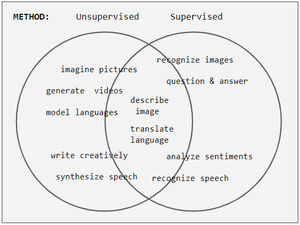
[2] Conceptually, unsupervised learning divides into the aspects of data, training, algorithm, and downstream applications.
This compares favorably to supervised learning, where the dataset (such as the ImageNet1000) is typically constructed manually, which is much more expensive.
In contrast to supervised methods' dominant use of backpropagation, unsupervised learning also employs other methods including: Hopfield learning rule, Boltzmann learning rule, Contrastive Divergence, Wake Sleep, Variational Inference, Maximum Likelihood, Maximum A Posteriori, Gibbs Sampling, and backpropagating reconstruction errors or hidden state reparameterizations.
This analogy with physics is inspired by Ludwig Boltzmann's analysis of a gas' macroscopic energy from the microscopic probabilities of particle motion
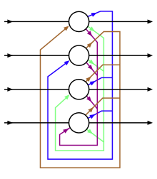
As network design changes, features are added on to enable new capabilities or removed to make learning faster.
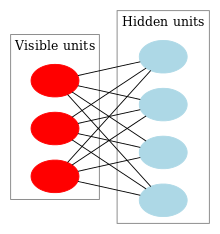
For instance, neurons change between deterministic (Hopfield) and stochastic (Boltzmann) to allow robust output, weights are removed within a layer (RBM) to hasten learning, or connections are allowed to become asymmetric (Helmholtz).
Boltzmann and Helmholtz came before artificial neural networks, but their work in physics and physiology inspired the analytical methods that were used.
The classical example of unsupervised learning in the study of neural networks is Donald Hebb's principle, that is, neurons that fire together wire together.
[8] In Hebbian learning, the connection is reinforced irrespective of an error, but is exclusively a function of the coincidence between action potentials between the two neurons.
[9] A similar version that modifies synaptic weights takes into account the time between the action potentials (spike-timing-dependent plasticity or STDP).
Among neural network models, the self-organizing map (SOM) and adaptive resonance theory (ART) are commonly used in unsupervised learning algorithms.
The SOM is a topographic organization in which nearby locations in the map represent inputs with similar properties.
The ART model allows the number of clusters to vary with problem size and lets the user control the degree of similarity between members of the same clusters by means of a user-defined constant called the vigilance parameter.
[10] Two of the main methods used in unsupervised learning are principal component and cluster analysis.
Cluster analysis is used in unsupervised learning to group, or segment, datasets with shared attributes in order to extrapolate algorithmic relationships.
[11] Cluster analysis is a branch of machine learning that groups the data that has not been labelled, classified or categorized.
This approach helps detect anomalous data points that do not fit into either group.
In particular, the method of moments is shown to be effective in learning the parameters of latent variable models.
It is shown that method of moments (tensor decomposition techniques) consistently recover the parameters of a large class of latent variable models under some assumptions.
[15] The Expectation–maximization algorithm (EM) is also one of the most practical methods for learning latent variable models.
However, it can get stuck in local optima, and it is not guaranteed that the algorithm will converge to the true unknown parameters of the model.