Visibility polygon
A visibility polygon is bounded if all rays shooting from the point eventually terminate in some obstacle.
In the latter case the visibility polygon may be found in linear time.
[1][2][3][4] Formally, we can define the planar visibility polygon problem as such.
For example, in robot localization, a robot using sensors such as a lidar will detect obstacles that it can see, which is similar to a visibility polygon.
[5] They are also useful in video games, with numerous online tutorials explaining simple algorithms for implementing it.
[6][7][8] Numerous algorithms have been proposed for computing the point visibility polygon.
For different variants of the problem (e.g. different types of obstacles), algorithms vary in time complexity.
In real life, a glowing point illuminates the region visible to it because it emits light in every direction.
Then, the pseudocode may be expressed in the following way: Now, if it were possible to try all the infinitely many angles, the result would be correct.
Unfortunately, it is impossible to really try every single direction due to the limitations of computers.
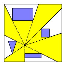
An approximation can be created by casting many, say, 50 rays spaced uniformly apart.
However, this is not an exact solution, since small obstacles might be missed by two adjacent rays entirely.
Furthermore, it is very slow, since one may have to shoot many rays to gain a roughly similar solution, and the output visibility polygon may have many more vertices in it than necessary.
The previously described algorithm can be significantly improved in both speed and correctness by making the observation that it suffices to only shoot rays to every obstacle's vertices.
This is sufficient for many simple applications such as video games, and as such many online tutorials teach this method.
, a linear time algorithm is optimal for computing the region in
In 1983, a conceptually simpler algorithm was proposed,[3] which had a minor error that was corrected in 1987.
The stack constitutes the vertices encountered so far which are visible to
If, later during the execution of the algorithm, some new vertices are encountered that obscure part of
vertices in total, it can be shown that in the worst case, a
[10] However, it relies on the linear time polygon triangulation algorithm by Chazelle, which is extremely complex.
segments that do not intersect except at their endpoints, it can be shown that in the worst case, a
This is because a visibility polygon algorithm must output the vertices of the visibility polygon in sorted order, hence the problem of sorting can be reduced to computing a visibility polygon.
A divide-and-conquer algorithm to compute the visibility polygon was proposed in 1987.
[12] An angular sweep, i.e. rotational plane sweep algorithm to compute the visibility polygon was proposed in 1985[13] and 1986.
[11] The idea is to first sort all the segment endpoints by polar angle, and then iterate over them in that order.
During the iteration, the event line is maintained as a heap.
[9] For a point among generally intersecting segments, the visibility polygon problem is reducible, in linear time, to the lower envelope problem.
By the Davenport–Schinzel argument, the lower envelope in the worst case has
A worst case optimal divide-and-conquer algorithm running in