Quadratic equation
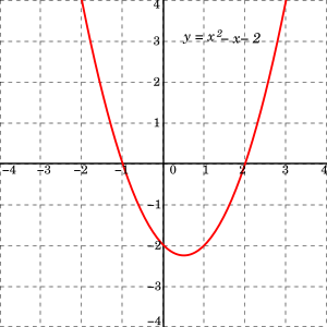
A quadratic equation whose coefficients are real numbers can have either zero, one, or two distinct real-valued solutions, also called roots.
A quadratic equation whose coefficients are arbitrary complex numbers always has two complex-valued roots which may or may not be distinct.
In some cases, it is possible, by simple inspection, to determine values of p, q, r, and s that make the two forms equivalent to one another.
The more general case where a does not equal 1 can require a considerable effort in trial and error guess-and-check, assuming that it can be factored at all by inspection.
This means that the great majority of quadratic equations that arise in practical applications cannot be solved by factoring by inspection.
[6]: 207 Starting with a quadratic equation in standard form, ax2 + bx + c = 0 We illustrate use of this algorithm by solving 2x2 + 4x − 4 = 0
Some sources, particularly older ones, use alternative parameterizations of the quadratic equation such as ax2 + 2bx + c = 0 or ax2 − 2bx + c = 0 ,[11] where b has a magnitude one half of the more common one, possibly with opposite sign.
These proofs are simpler than the standard completing the square method, represent interesting applications of other frequently used techniques in algebra, or offer insight into other areas of mathematics.
In this case, the subtraction of two nearly equal numbers will cause loss of significance or catastrophic cancellation in the smaller root.
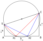
Descartes' theorem states that for every four kissing (mutually tangent) circles, their radii satisfy a particular quadratic equation.
[19] In modern notation, the problems typically involved solving a pair of simultaneous equations of the form:
The steps given by Babylonian scribes for solving the above rectangle problem, in terms of x and y, were as follows: In modern notation this means calculating
with a = 1, b = −p, and c = q. Geometric methods were used to solve quadratic equations in Babylonia, Egypt, Greece, China, and India.
With a purely geometric approach Pythagoras and Euclid created a general procedure to find solutions of the quadratic equation.
Muhammad ibn Musa al-Khwarizmi (9th century) developed a set of formulas that worked for positive solutions.
[27] He also described the method of completing the square and recognized that the discriminant must be positive,[27][28]: 230 which was proven by his contemporary 'Abd al-Hamīd ibn Turk (Central Asia, 9th century) who gave geometric figures to prove that if the discriminant is negative, a quadratic equation has no solution.
[30] The 9th century Indian mathematician Sridhara wrote down rules for solving quadratic equations.
[31] The Jewish mathematician Abraham bar Hiyya Ha-Nasi (12th century, Spain) authored the first European book to include the full solution to the general quadratic equation.
[27] The writing of the Chinese mathematician Yang Hui (1238–1298 AD) is the first known one in which quadratic equations with negative coefficients of 'x' appear, although he attributes this to the earlier Liu Yi.
[34] In 1637 René Descartes published La Géométrie containing the quadratic formula in the form we know today.
The figure shows the difference between[clarification needed] (i) a direct evaluation using the quadratic formula (accurate when the roots are near each other in value) and (ii) an evaluation based upon the above approximation of Vieta's formulas (accurate when the roots are widely spaced).
However, at some point the quadratic formula begins to lose accuracy because of round off error, while the approximate method continues to improve.
This situation arises commonly in amplifier design, where widely separated roots are desired to ensure a stable operation (see Step response).
Methods of numerical approximation existed, called prosthaphaeresis, that offered shortcuts around time-consuming operations such as multiplication and taking powers and roots.
[35] Astronomers, especially, were concerned with methods that could speed up the long series of computations involved in celestial mechanics calculations.
It is within this context that we may understand the development of means of solving quadratic equations by the aid of trigonometric substitution.
Substituting the two values of θn or θp found from equations [4] or [5] into [2] gives the required roots of [1].
Complex roots occur in the solution based on equation [5] if the absolute value of sin 2θp exceeds unity.
[37] To illustrate, let us assume we had available seven-place logarithm and trigonometric tables, and wished to solve the following to six-significant-figure accuracy:
The formula and its derivation remain correct if the coefficients a, b and c are complex numbers, or more generally members of any field whose characteristic is not 2.