Interval arithmetic

Numerical methods involving interval arithmetic can guarantee relatively reliable and mathematically correct results.

The latter often arise from measurement errors and tolerances for components or due to limits on computational accuracy.

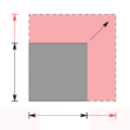
The main objective of interval arithmetic is to provide a simple way of calculating upper and lower bounds of a function's range in one or more variables.

BMI is calculated as a person's body weight in kilograms divided by the square of their height in meters.

Suppose a person uses a scale that has a precision of one kilogram, where intermediate values cannot be discerned, and the true weight is rounded to the nearest whole number.

Since the BMI uniformly increases with respect to weight and decreases with respect to height, the error interval can be calculated by substituting the lowest and highest values of each interval, and then selecting the lowest and highest results as boundaries.

is monotone for each operand on the intervals, which is the case for the four basic arithmetic operations (except division when the denominator contains

For sine and cosine, only the endpoints need full evaluation, as the critical points lead to easily pre-calculated values—namely -1, 0, and 1.

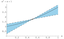
Tighter extensions are desirable, though the relative costs of calculation and imprecision should be considered; in this case,

One can either define complex interval arithmetic using rectangles or using disks, both with their respective advantages and disadvantages.

The earlier operations were based on exact arithmetic, but in general fast numerical solution methods may not be available for it.

This replaces the numerical operations, in that the linear algebra method known as Gaussian elimination becomes its interval version.

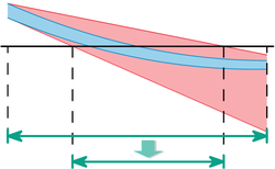
Hence using the result of the interval-valued Gauss only provides first rough estimates, since although it contains the entire solution set, it also has a large area outside it.

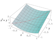
are invertible, it is sufficient to consider all possible combinations (upper and lower) of the endpoints occurring in the intervals.

Parameters for which no exact figures can be allocated often arise during the simulation of technical and physical processes.

Unlike point methods, such as Monte Carlo simulation, interval arithmetic methodology ensures that no part of the solution area can be overlooked.

Rules for calculating with intervals and other subsets of the real numbers were published in a 1931 work by Rosalind Cicely Young.

A comprehensive paper on interval algebra in numerical analysis was published by Teruo Sunaga (1958).

Independently in 1956, Mieczyslaw Warmus suggested formulae for calculations with intervals,[15] though Moore found the first non-trivial applications.

For example, Karl Nickel [de] explored more effective implementations, while improved containment procedures for the solution set of systems of equations were due to Arnold Neumaier among others.

In 1988, Rudolf Lohner developed Fortran-based software for reliable solutions for initial value problems using ordinary differential equations.

As lead editor, R. Baker Kearfott, in addition to his work on global optimization, has contributed significantly to the unification of notation and terminology used in interval arithmetic.

Since 1967, Extensions for Scientific Computation (XSC) have been developed in the University of Karlsruhe for various programming languages, such as C++, Fortran, and Pascal.

There followed in 1976, Pascal-SC, a Pascal variant on a Zilog Z80 that it made possible to create fast, complicated routines for automated result verification.

Starting from 1991 one could produce code for C compilers with Pascal-XSC; a year later the C++ class library supported C-XSC on many different computer systems.

At the beginning of 2000, C-XSC 2.0 was released under the leadership of the working group for scientific computation at the Bergische University of Wuppertal to correspond to the improved C++ standard.

[28] In addition, computer algebra systems, such as Euler Mathematical Toolbox, FriCAS, Maple, Mathematica, Maxima[29] and MuPAD, can handle intervals.

A Matlab extension Intlab[30] builds on BLAS routines, and the toolbox b4m makes a Profil/BIAS interface.

[34] These have been developed by members of the standard's working group: The libieeep1788[35] library for C++, and the interval package[36] for GNU Octave.

A minimal subset of the standard, IEEE Std 1788.1-2017, has been approved in December 2017 and published in February 2018.